College Admissions as Non-Price Competition: The Case of South Korea

NBER WORKING PAPER SERIES

COLLEGE ADMISSIONS AS NON-PRICE COMPETITION:

THE CASE OF SOUTH KOREA

Christopher Avery

Soohyung Lee

Alvin E. Roth

Working Paper 20774

http://www.nber.org/papers/w20774

NATIONAL BUREAU OF ECONOMIC RESEARCH

1050 Massachusetts Avenue

Cambridge, MA 02138

December 2014

Roth’s work was partially supported by NSF Grant 1061889. The views expressed herein are those

of the authors and do not necessarily reflect the views of the National Bureau of Economic Research.

At least one co-author has disclosed a financial relationship of potential relevance for this research.

Further information is available online at http://www.nber.org/papers/w20774.ack

NBER working papers are circulated for discussion and comment purposes. They have not been peer-

reviewed or been subject to the review by the NBER Board of Directors that accompanies official

NBER publications.

of text, not to exceed two paragraphs, may be quoted without explicit permission provided that full

credit, including © notice, is given to the source.

College Admissions as Non-Price Competition: The Case of South Korea

Christopher Avery, Soohyung Lee, and Alvin E. Roth

NBER Working Paper No. 20774

December 2014

JEL No. C78,I23

ABSTRACT

This paper examines non-price competition among colleges to attract highly qualified students, exploiting

the South Korean setting where the national government sets rules governing applications. We identify

some basic facts about the behavior of colleges before and after a 1994 policy change that changed

the timing of the national college entrance exam and introduced early admissions, and propose a game-

theoretic model that matches those facts. When applications reveal information about students that

is of common interest to all colleges, lower-ranked colleges can gain in competition with higher-ranked

colleges by limiting the number of possible applications.

Christopher Avery

Harvard Kennedy School of Government

79 JFK Street

Cambridge, MA 02138

and NBER

[email protected]

Soohyung Lee

Department of Economics

University of Maryland

3147B Tydings Hall

College Park, MD 20742

[email protected]

Alvin E. Roth

Department of Economics

Stanford University

579 Serra Mall

Stanford, CA 94305

and NBER

[email protected]

A data appendix is available at:

http://www.nber.org/data-appendix/w20774

2

I. Introduction

College admissions is a matching market, in which applicants cannot simply choose what

college to attend, even if they can afford it, but in which they must also be admitted.

That is, prices are not used to equate supply and demand: selective colleges are priced to

attract many more students than they can admit, and admissions policies thus serve to

clear the market. Compared to the immense interest in college admissions in the press,

relatively little academic research on this topic has been conducted in the field of

economics. One reason may be that while college admissions processes are complex,

only partial information is available for analysis.

This paper utilizes a setting with a well-defined set of strategies for colleges and

where relevant information is available, namely South Korea, where the central

government determines the total number of seats a college can fill in an incoming cohort

and the methods by which a college can evaluate its applicants. These centralized rules

governing the admissions process allow us to model and analyze the strategic decisions

of South Korean colleges more precisely than would be possible in the decentralized

environment in which American colleges operate.

We focus on recent changes in the rules and timing for college admissions in

South Korea, and in particular, on a set of reforms that introduced early applications in

1994.

1

Between 1982 and 1993, the national exam required for college admission in

South Korea was only offered on two dates each year, and students were allowed to apply

for only one college per exam date.

2

Thus, there was a structural limitation of at most

two applications per student. In addition, many of the most selective colleges, including

all of the top nine by a common reputational ranking (see Table 1), chose to fill their

classes on the first exam date. That is, students were able to apply to at most one very

selective college, since those colleges all held their examinations on the same day and

since a student could only apply to a college where he or she took the exam.

Limitations on the ability of students and colleges to explore possible matches

typically lead to inefficiencies characteristic of “congested” markets, when participants

1

By 1994, we mean the policy change applied to the cohort who entered colleges from the 1994 academic

year (March 1994).

2

We refer to a 4-year post secondary institute as a college except when it is part of the proper name of an

institution. Such a college is typically referred to as a university in South Korea.

3

are unable to “consider enough alternative possible transactions to arrive at satisfactory

ones” (Roth, 2008). Congestion frequently leads to unstable matches and subsequent

pressure to change the rules of the matching system (see for example Roth and Xing,

1997). In South Korea, it became common for students who were not admitted to their

first-choice colleges to wait another year and participate in the next admissions cycle

rather than to enroll immediately at a second (or worse) choice college.

Partly to address this obvious inefficiency, the South Korean government changed

the admission rules in 1994 to allow multiple applications, including a first phase

officially designated as an early application period. This reform also introduced a

centralized date for the national examination during the early application period, thereby

allowing colleges to create and offer idiosyncratic and specialized examinations during

the regular application period. That is, after the reform the national exam was

administered to all students before the start of [early] applications, thereby allowing

colleges to develop additional individualized exams to further differentiate applicants

during the regular admissions process.

In this paper, we develop a model to study the incentives for colleges under these

two regimes and compare the predictions of the model to stylized facts about the behavior

of South Korean colleges given each set of rules. We then assess the success of the

reform using aggregated data on the number of re-applicants before and after these

changes to admissions rules.

Our analysis is related to several papers in the economics literatures on matching

and college admissions. Chen and Kao (2014a, 2014b) develop related models of

graduate school admissions in Taiwan to make the point that a second-ranked college can

gain from a “single application rule” if that would enable it to draw applicants away from

a top-ranked college. This result is quite similar in nature to Proposition 2 in this paper,

though our model is more general than that of Chen and Kao. Che and Koh (2014) study

the relationship between competition and coordination in admission policies of

competing colleges who are especially concerned about over-enrollment or under-

enrollment, finding that colleges have incentives to develop negatively correlated

admissions practices. Though they do not emphasize this point, the Che and Koh model

suggests that colleges might opt for a single application rule in order to reduce

4

uncertainty about total enrollment.

3

The competitive advantage gained by the less

preferred college in a single application system is reminiscent of strategic gains to lower

ranked colleges from early application programs in the United States (Avery and Levin

(2010), Avery, Fairbanks, and Zeckhauser (2003)). Hafalir et al. (2014) compare

centralized admissions, by exam, in which students effectively can apply to all colleges,

with an alternative regime in which each student is restricted to apply to only one college.

They show that when students must decide how much costly effort to commit to the

admissions process, higher ability students prefer centralized admissions in this model.

Our model is also quite related in structure to the model of Chade, Lewis, and

Smith (2014) (we refer to this paper below as CLS), who study the application choices of

students considering two colleges, where one college is universally agreed to be

preferable to the other. The primary difference between our paper and CLS is in focus.

CLS is oriented towards “application portfolios”, especially the value of applying to both

colleges rather than just one of them. By contrast, we are interested in the current paper

about the strategic choices of the colleges to expand or contract application options for

students. That is, we consider the situation facing colleges whose strategies interact to

determine both the timing of applications and the number of applications that a student

can submit.

The paper proceeds as follows. Section II provides additional background on the

nature and history of South Korean college admissions. Section III describes the

theoretical model. Section IV reports the results of equilibrium analysis and suggests a

series of empirical hypotheses to test. Section V concludes.

3

This was precisely the motivation for an earlier reform in 1982 in South Korea that limited students to no

more than two applications under the rules described above. Prior to 1982, South Korean students could

apply to an unlimited number of colleges, but it was felt that colleges faced burdensome administrative

costs for keeping track of their waiting lists under those rules. (see Hwang, 1994)

5

II. Background on South Korean College Admissions

Graduating from a prestigious college is an effective and popular way for a South Korean

to improve his/her status (Sorensen 1994, and Lee 2007).

4

Competition among students

is intense to gain admission to a prestigious college, and many high school graduates are

willing to spend an extra year in prep school in order to get an extra chance to apply to a

highly ranked college. Perhaps because of this intense social interest in college choice,

the South Korean government has been deeply involved in designing college admissions

systems and regulating the admissions policies of both public and private colleges.

College rankings are fairly well-agreed upon among South Koreans and stable

across time, which can be shown from the quality of applicants to each college and from

evaluation by third party agencies similar to the US News and World Report annual

rankings. Seoul National University (herein, Seoul National) is considered the best,

followed by the second group of colleges, which includes Yonsei, Korea, KAIST, and

Postech. The third group of colleges, considered to rank right below these four colleges,

includes Sogang, Hanyang, Seongkyunkwan, Ewha, Pusan, Kyungbook, Hankook

Foreign Language, Joongang, and Kyunghee universities.

5

See Online Appendix 1.1 for

details.

From 1982 to 1993, the South Korean government conducted national exams

twice a year and required all colleges to make admissions decisions according to a

composite index based on the nationwide exam score and high school performance.

6

After some year-to-year modifications from 1982 to 1987, the Korean government settled

on a stable set of rules that were in place from 1988 to 1993, as shown in Panel A of

Figure 1.

In this system, the South Korean government announced the two exam dates

(typically one in January, the other in February) and then colleges announced how they

4

Lee (2007) reports that in 2003, 48 percent of the CEOs of the Hankyung’s top 81 South Korean firms

had been undergraduates at Seoul National University (which accounts for only 0.4 percent of South

Korean college graduates) and that an additional 26 percent of CEOs of these firms were undergraduates at

Yonsei or Korea University. By contrast, he finds that in 2004, 17 percent of CEOs of S&P 500 firms were

graduates of the top ten ranked colleges in the United States.

5

These rankings refer only to the main campuses of these colleges. Several of these top 13 ranked colleges

have additional affiliated campuses that typically operate independently and have much lower prestige.

6

In theory, colleges were allowed to conduct interviews and to include the results as up to 10 percent of the

composite index. In practice, however, such interviews had little effect on admission decisions (Hwang,

1994).

6

Figure 1 Time Line

Panel A: 1988 to 1993 Academic Year

Date 1/

National Exam 1

Date 2/

National Exam 2

15-Nov

1-Dec

1-Jan

1-Feb

Panel B: 1994 to 2001 Academic Year

National

Exam

Score

Release

Regular Admission

15-Nov

1-Dec

Early

Admission

1-Jan

1-Feb

would allocate their seats between the two exam dates at the beginning of the academic

year. Each student was restricted to a maximum of two applications, one per national

examination date. Each application specified a single program of study at a particular

college and the candidate was required to take the exam at that particular college as part

of the application. In practice, Date 1 (early January) had the flavor of “early decision”

in the United States system, because students were required to enroll if admitted in that

round, while Date 2 (February) had the flavor of a last-chance “scramble.” Since most

high-ranked colleges allocated all of their seats to Date 1, in essence, students could only

apply to a single program at a high-ranked college.

7

In 1994 the South Korean government introduced a series of reforms for

applications. These reforms had three major goals: (1) changing the format of the

national exam to emphasize complex reasoning skills rather than memorization; (2)

promoting the autonomy of individual colleges in admissions decisions by allowing

7

Similarly, in the United Kingdom, applicants are restricted to a single application to either Cambridge or

Oxford University. Further, this application must specify a particular college (one of the more than 60

colleges at the two universities) and a particular program of study at that college.

http://www.ucas.com/how-it-all-works/undergraduate/filling-your-application

7

institution-specific examinations in part of the admissions process; (3) providing more

application options for students to reduce the number of students enrolling in prep school

and applying again the following year.

8

These new rules changed the timing and location of the national exam, introduced

a system of early admissions, expanded the number of possible regular admission dates

from two to four, and allowed each college to administer a specialized exam as part of a

regular application. Under the rules of the revised system, students first took the

nationwide exam at a neighborhood public school in mid-November and learned their

scores prior to submitting an application to any college. As in the previous system, each

application was to a single program of study at a particular college. Colleges specified

how many seats in the entering class to allocate to early admission (it was possible to

choose not to participate in early admissions by allocating zero seats to it) and then

allocated all remaining seats across the four regular application dates.

Panel B of Figure 1 shows the timeline that was in place after the introduction of

early applications in 1994. Once a student received his/her test score on the nationwide

exam, he/she decided whether to submit an early application (in mid-December) to a

college that offered early admission. Early admission was binding in that a student could

apply early to only one school, and was required to enroll if admitted. A student

participating in regular admissions could apply to up to four schools (one school per

regular admission date) and could choose from among those that admitted him/her.

9

One

important difference between early and regular admission was that students took a

specialized exam at each college to which they applied as regular applicants, whereas

early admission was based only on high school grades and scores on the national exam.

8

The original documents are in Korean and are available at the national archive of official government

documents at http://contents.archives.go.kr. We also consulted a 1998 technical report from the South

Korean Ministry of Education, “50 Years of Korean Education Policies”. Weidman and Park (2000) for an

overview of the South Korean college admission system written in English.

9

There were policy debates over providing students even more opportunities for college applications

instead of giving them up to 5 chances (early admission and four applications in regular admission).

However, there was major resistance from colleges, based on several concerns, including the possibility of

“losing face,” “congestion,” and lack of applications to low-ranked colleges.

(http://magazine.kcue.or.kr/last/popup.html?vol=99&no=476

http://www.snujn.com/site/art_view.html?id=878) There may also have been some institutional memory of

the problems with the system prior to 1982, when students were allowed to apply to an unlimited number of

colleges.

8

In part for this reason, a student who applied but was not admitted to a particular program

as an early applicant could apply again to that same program in regular admissions.

In 2002, the government changed the application system in an attempt to promote

diversity in enrollment. Early applications were limited to students who met particular

eligibility criteria, such as qualifying for the Math Olympiad or residing in an

underrepresented rural area. Although it was not stated explicitly, it seems plausible that

this reform was intended to limit the importance of early applications. However, since

the criteria for eligibility were set individually by each college, the program quickly

expanded to include a wide range of applicants, as we discuss below. The rules for

regular admissions have been largely unchanged from 1994 to the present, though today

there are three rather than four possible dates for regular applications.

This paper focuses on the admission policies of 13 elite colleges between 1993

and 2001. While we do not study the policies of these colleges in detail beyond 2001, we

view the evolution of their strategies between 2002 and the present as largely consistent

with the results for the system between 1993 and 2001, as we describe in the discussion

of Tables 2, 3, and 4 below.

We collected the information released by the Korean Council for University

Education (KCUE) and by Seoul National and all colleges in Groups 2 and 3, excluding

KAIST.

10

We omit KAIST because it is exempt from the government’s college admission

policy in that in addition to high school seniors (12

th

graders), it can accept 11

th

graders

enrolled in science high schools without a nationwide test score.

10

For each admission cycle, we collected press releases by those colleges every year, reported in 5 major

South Korean newspapers. Such press releases include the information of the total seats, and the allocation

of seats across exam dates and early application. For each college and year, we crosscheck the accuracy of

the information by checking two to three different major newspapers.

9

II.A Stylized Facts

This information suggests the following stylized facts.

(F1) Prior to the policy change in 1994, almost all elite colleges chose the same date

(Date 1) for the national exam and admissions.

Table 1 shows the number of seats each college can fill up to and the fraction of seats

allocated between Dates 1 and 2 in 1993. For example, Seoul National, Korea, Yonsei,

and Postech selected their students entirely from Date 1, as did the majority of the group

3 colleges. Although several colleges selected students from both Dates 1 and 2, they still

filled the majority of their seats on Date 1.

Table 1 Distribution of Seats Before the Policy Change (1993)

Group

College

Seats

Date 1

Date 2

1

Seoul National

4,905

100%

0%

2

Korea

3,930

100%

0%

Yonsei

3,930

100%

0%

Postech

300

100%

0%

3

Sogang

1,700

100%

0%

Ewha women’s

3,670

100%

0%

Pusan

4,370

100%

0%

Kyungbook

4,370

100%

0%

Joongang

2,315

100%

0%

Hanyang

3,320

79%

21%

Kyunghee

2,000

77%

23%

Seongkyunkwan

3,850

69%

31%

Hankook

1,730

50%

(F2) After the policy change in 1994, schools just below the very top chose a different

(regular) admissions date than the date chosen by the top-ranked school, Seoul National.

Although the government specified four separate possible dates for regular admissions,

most of the top-ranked colleges chose a single date for regular admissions in each year

during this time period. For example, in 1994 and 1995, all 13 colleges conducted

regular admissions on just a single date, though not all chose the same date. Similarly, in

2000 and 2001, 10 of these 13 colleges conducted regular admissions on just a single date

10

and two of the others offered a clear majority (between 70 and 100 percent) of their

regular admissions seats on a single date.

Table 2 identifies the date for which each of these 13 colleges offered the majority

of its regular admissions seats from 1994 to 2001. (See Online Appendix 1.2 for the

exact percentages of seats offered by each college in each year.) In the first two years

after the policy change, 10 of these 13 colleges continued their pre-existing practice of

emphasizing “Date A”, the regular admissions date chosen by Seoul National.

11

However, in 1996, the third year after the reform, seven of these colleges switched from

“Date A” to “Date B”. From that point on, none of the Group 2 colleges and at most 3 of

the 9 Group 3 colleges offered “Date A” as its primary date for regular admissions.

Despite the small sample size, this reduction from 75% in 1995 to 25% in 2001 of Group

2 and Group 3 colleges offering “Date A” as the primary regular admissions date is

statistically significant at the 5% level in a simple two-sample Binomial comparison.

Table 2 Choice of Regular Exam Dates since 1994

1994

1995

1996

1997

1998

1999

2000

2001

A

B

C

A

B

C

A

B

C

A

B

C

A

B

C

A

B

C

A

B

C

A

B

C

1

Seoul National

*

2

Korea

*

Yonsei

*

Postech

*

3

Sogang

*

Ewha women’s

*

Pusan

*

Kyungbook

*

Joongang

*

Hanyang

*

Kyunghee

*

Seongkyunkwan

*

Hankook

*

11

For simplicity in presentation, we define “Date A” as the regular admissions date chosen by Seoul

National University, “Date B” as the regular admissions date chosen by Postech, and “Date C” as a

combination of the remaining two regular admissions dates specified by the government.

11

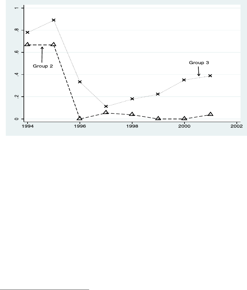
Figure 2 plots the average percentages of regular admissions seats allocated to

Date A in each group and year, weighting each college equally.

12

From 1996 to 2001, a

negligible fraction of regular admission seats were allocated to Date A in Group 2. For

Group 3, the average fraction of regular admissions seats allocated to Date A decreased

from over 80 percent to less than 40 percent in 1996 and then settled around 30 percent.

Figure 2 Regular Admission: Fraction of Seats Allocated to Date A (Seoul National)

(F3) Early applications gained steadily in importance from 1994 to 2001. Seoul

National, the top-ranked college, was among the last colleges to adopt early admissions.

Table 3 presents the share of seats each college allocated to early admission in each year

from 1994 to 2001. Although 10 of the 12 competitors to Seoul National adopted early

admissions immediately after the reform in 1994, they initially offered proportionally few

seats to early applicants, and only one of them, Postech, enrolled 40 percent of its

entering class early that year. All twelve of these colleges increased their use of early

admissions over time, and by 2001, Hanyang was the only one that enrolled less than 40

percent of its entering class early. As a group, these 12 colleges almost tripled their use

of early admissions between 1994 and 2001, offering an average of 16.8% of their seats

12

The results are similar if we use a weighted average based on the number of seats offered by each

college.

12

Table 3 Percent of Seats Allocated to Early Admission since 1994

1994

1995

1996

1997

1998

1999

2000

2001

1

Seoul National

0

19

18

20

2

Korea

24

30

37

46

41

49

54

Yonsei

19

37

41

50

53

59

60

57

Postech

40

51

40

50

56

3

Sogang

25

30

40

49

35

41

44

46

Ewha women’s

12

32

33

44

49

48

Pusan

0

6

27

43

47

43

Kyungbook

0

9

27

48

50

49

53

Joongang

9

35

34

45

31

33

44

46

Hanyang

18

26

35

41

45

43

42

37

Kyunghee

22

13

38

46

44

41

Seongkyunkwan

13

32

38

41

36

45

44

47

Hankook

20

39

30

28

24

39

46

40

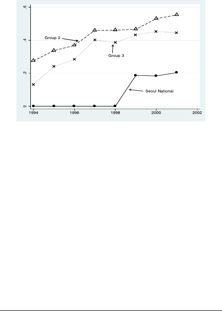
Figure 3 graphs the fraction of seats allocated to early admission by group and

year. The percentage of seats offered to early applicants by both Group 2 and Group 3

colleges increased fairly steadily over time, and by 1999 colleges in both groups were

offering an average of more than 40 percent of their seats to early applicants.

Interestingly, Seoul National began offering early admissions only in 1999, after its

primary competitors were already emphasizing early admissions to a considerable degree.

This choice mirrors changes in early admission practice in the United States, where

Harvard and Princeton eliminated their early application programs in 2006, but then

reinstated them in 2011. Administrators from both these colleges explained a primary

reason for this change in 2011 was that not offering early applications was putting their

institutions at a competitive disadvantage. For example, Michael Smith, Dean of the

Faculty of Arts and Sciences at Harvard, commented: “We looked carefully at trends in

Harvard admissions these past years and saw that many highly talented students,

including some of the best-prepared low-income and underrepresented minority students,

were choosing programs with an early-action option, and therefore were missing out on

the opportunity to consider Harvard”.

13

“Early Action Returns,” Harvard Gazette, February 24, 2011,

http://news.harvard.edu/gazette/story/2011/02/early-action-returns/. See also “Princeton to Reinstate Early

Admissions Program,” Feburary 24, 2011, http://www.princeton.edu/main/news/archive/S29/85/15K32/

13

Figure 3 Percentage of Seats Offered Through Early Admission

Although we do not have direct evidence about the decision of Seoul National to offer

early admissions for the first time in 1999, the circumstantial evidence suggests that it did

so in response to competitive pressure. Interestingly, it appears that its competitors

responded by emphasizing early admission to an even greater degree. The three Group 2

competitors to Seoul National offered an average of 46 percent of seats to early

applicants in 1997, 1998, and 1999, but then increased this percentage to 53 and 56

percent in 2000 and 2001, the two years after Seoul National first offered early

admissions.

(F4) The rule change in 2002 had little effect on the prevailing trends in admission

practice. Early admissions has continued to grow in importance to the present, while

schools just below the very top continue to choose a different (regular) admissions date

than the date chosen by the top-ranked school, Seoul National.

Table 4 presents the share of seats each college allocated to early admission and to each

of the regular admission dates in 2014 and 2015. Whereas these colleges allocated an

average of 45 percent of seats to early applicants in 2000 and 2001, they now allocate an

14

average of 68 percent of seats to early applicants today. In addition, the second-tier

colleges, Korea and Yonsei continue to choose a different regular admission date than the

top ranked college, Seoul National.

Table 4 Percent of Seats Allocated to Admission/Exam Days: 2014 and 2015

2014

2015

Early

Regular

Early

Regular

A

B

C

A

B

C

1

Seoul National

82

18

0

75

25

0

2

Korea

69

0

31

0

71

0

29

0

Yonsei

55

0

45

0

64

0

36

0

Postech

100

0

100

0

3

Sogang

69

31

0

62

38

0

Ewha women’s

64

0

36

0

62

38

0

Pusan

61

20

19

0

55

23

0

Kyungbook

62

19

20

0

57

21

22

0

Joongang

72

14

12

3

69

18

12

2

Hanyang

71

9

20

0

78

6

15

0

Kyunghee

56

25

14

6

61

19

20

0

Seongkyunkwan

69

12

18

0

76

10

14

0

Hankook

60

14

8

17

54

9

23

13

(F5) The 1994 reform somewhat reduced, but by no means eliminated the phenomenon

of repeat applications.

Table 5 lists the number of high school seniors and repeat applicants to (all) four-year

colleges in South Korea from 1990 to 2001. An average of 318,543 students – more than

half of the high school seniors from the prior year

14

- were repeat applicants each year in

the four years prior to the reform. In 1994, the first year after the reform, there was an

immediate drop of about 25% in the number of repeat applicants, but some potential

repeat applicants may have been discouraged by the change in format of the national

exam that went along with the reform. After excluding 1994, there were an average of

260,288 repeat applicants per year from 1995 to 2001, or about an 18 percentage point

decline per year from the four years just prior to the reform. Despite the small sample

14

This computation assumes that students reapply at most once, which is not necessarily the case.

15

size, this decline in the absolute number of repeat applicants on average per year before

and after the 1994 reform is significant at the 1% level in a two sample t-test.

Table 5 Fraction of Repeat Applicants

Year

No. High

School

Seniors

No. Repeat

Applicants

Total Seats

in College

Admission

Overall

Competition

[(1)+(2)]/(3)

% of Repeat

Applicants

(2)/[(1)+(2)]

% of Repeat

relative to previous

year’s non-admits

(2)

t

/[(1)+(2)-(3)]

t-1

(1)

(2)

(3)

(4)

(5)

(6)

1990

597,456

283,890

199,380

4.420

32.2

-

1991

610,586

331,212

204,995

4.594

35.2

48.6

1992

594,500

336,861

215,565

4.321

36.2

45.7

1993

602,144

322,208

224,159

4.124

34.9

45.0

1994

526,703

248,102

236,653

3.274

32.0

35.4

1995

492,471

276,262

257,859

2.981

35.9

51.3

1996

528,690

300,546

271,015

3.060

36.2

58.8

1997

546,172

265,817

298,328

2.722

32.7

47.6

1998

612,379

245,791

304,265

2.820

28.6

47.9

1999

622,964

231,072

311,590

2.741

27.1

41.7

2000

632,171

248,930

337,721

2.609

28.3

45.9

2001

603,224

253,601

339,209

2.526

29.6

46.7

Two demographic changes complicate the analysis of pre- and post-reform data.

First, Table 5 indicates a conspicuous decline in the number of high school seniors from

1993 to 1994-1997, the first four years after the reform. It would be predictable,

presumably with a one-year lag, to find fewer repeat applicants in this period when there

were fewer new applicants than the pre-reform period. The decline in the number of high

school seniors eventually reversed, however, and there were even more high school

seniors in each year from 1998 to 2000 (and almost as many in 2001) as in any year from

1990 to 1993. Further, there were even fewer repeat applicants in this period from 1998

to 2001 than in the first four years after the reform.

15

Second, Table 5 indicates that the total admission seats available increased every

year during the sample period, resulting in an increase in more than 50% in available

places from 1990 to 2001. Presumably, this expansion of admission seats would yield a

15

Restricting the post-reform sample to 1998 to 2001, with or without incorporating a one year lag for

repeat applicants to appear in the data, we still find a significant decline in the absolute number of repeat

applicants per year by comparison to the pre-reform years of 1990 to 1993.

16

result where more students would be placed in desirable college seats each year – if so, it

would be predictable to find fewer repeat applicants in subsequent years as a result. One

straightforward approach to account for the expansion of admission seats is to find the

ratio of repeat applicants in one year to the number of applicants who applied the

previous year but did not enroll (the difference between total number of applicants and

total number of seats).

16

By this approach, we find only a very small (and clearly

insignificant) change as a result of the reform: 46.4 percent of unmatched students in

1990 to 1992 and 44.7 percent of unmatched students in 1998 to 2000 returned as repeat

applicants the following year. At the same time, this approach presumably overstates the

importance of the expansion of seats, for it is likely that the new seats were

disproportionately placed at low-ranked colleges and that many of them were not filled.

Taking these observations together, we find little evidence that the reduction in

the number of repeat applicants after the 1993 reform could be explained by changes in

the number of high school seniors each year, but it is possible that the expansion of the

number of places in colleges could explain at least some of this reduction.

III. The Model

Suppose that there are two colleges and a continuum of ex ante identical students. All

students have identical preferences with utility u

1

= 1 for attending College 1 and utility

u

2

for attending College 2, where 0 < u

2

< 1. Each college wishes to enroll the same

proportion K < ½ of all students. Applications are costless, so if possible, each student

applies to both colleges.

At the start of the application process, the only information differentiating one

student from another is high school grade point average, which we denote by x

i

for

student i. During the application process, each student takes the national college entrance

exam and we denote student i’s score on this exam by s

i

. We assume further that colleges

agree on a subsequent ranking of students based on an index, y

i

= y(x

i

, s

i

), which

summarizes the information contained in high school grades and the national exam score,

with all values x

i

, s

i

, y

i

scaled to range from 0 to 1.

Student i provides utility vij to the college by enrolling at college j, where vij

16

This computation assumes that all available seats are filled in a given year by applicants from that year.

17

ranges from 0 to 1 . We assume that a student’s grades, x

i

, national exam score s

i

, and

specialized exam score s

ij

at college j (if available) s

ij

combine to identify v

ij

= z(y

i

, s

ij

),

where z is continuous, differentiable and strictly increasing in each argument, while s

i1

and s

i2

are identically distributed and conditionally independent given x

i

and s

i

.

17

We

further assume that there is a joint distribution of values f(x

i

, s

i

, v

ij

) such that the

conditional distributions g(y

i

| x

i

) and h(v

ij

| y

i

) satisfy the strict monotone likelihood ratio

property: for y

i

< y

i

’ and v

ij

> v

ij

’

h(v

ij

| y

i

) / h(v

ij

’ | y

i

) > h(v

ij

| y

i

’) / h(v

ij

’ | y

i

’).

Similarly, for x

i

> x

i

’, y

i

> y

i

’,

g(y

i

| x

i

) / g(y

i

’ | x

i

) > g(y

i

| x

i

’) / g(y

i

’ | x

i

’).

To rule out boundary issues, we assume that all possible pairwise combinations of

GPA and national test score, national test score and specialized exam score take strictly

positive densities: f(x

i

, s

i

, s

ij

) >  for each (x

i

, s

i

, s

ij

) and similarly g(y

i

| x

i

) >  for each

(x

i

, y

i

); h(v

ij

| y

i

) >  for each (y

i

, v

ij

), where  is a known positive constant.

We use this general framework to study the incentives for colleges and students

using equilibrium analysis for each of two different sets of rules. We label the initial set

of rules, which were in place until 1994, as “Regime 1”. In Regime 1, we assume that

student i knows x

i

at the start of the admissions process, prior to submitting any

applications, and that admissions decisions at each college are based on y

i

values.

College 1 moves first and announces which one of the two possible dates it will offer.

Then College 2 responds by announcing its choice of the two possible admission dates.

Once the colleges have announced their admission timetables, students decide which

college to apply to on the first date and the admissions process moves along accordingly

from there. Any student admitted on Date 1 must attend the college where he/she

applied; a student who was not admitted on Date 1 can apply again on Day 2. We prove

17

The assumption that s

i1

and s

i2

are conditionally independent given x

i

and s

i

essentially means that the

specialized exam score at one college is not relevant to the student’s likely performance at the other

college. We make this extreme assumption to emphasize the differential implications of (1) common

information about a student’s underlying academic preparation and (2) idiosyncratic information about the

value of a student-college match for the strategies selected by colleges.

18

in Online Appendix 3 that Proposition 2, the key result for Regime 1, also holds in the

case where each college can admit some students on each date.

18

We label the new system, which was put in place in 1994 as “Regime 2”. In

Regime 2, we assume that student i knows y

i

at the start of the admissions process, prior

to submitting any applications, that early admissions decisions at each college are based

on y

i

and that regular admissions decisions at college j are based on v

ij

values (as

revealed by specialized exams at each college). College 1 moves first and announces

both the number of students it will admit early and the regular admissions date it will use

to fill the remainder of its entering class, then College 2 responds by announcing its

allocation of seats to early and regular admissions along with its regular admissions date.

Once these admission schedules are announced, students decide whether to apply early to

one college and the admissions process moves along accordingly from there. In this

regime, early application is binding, so that any student admitted early must attend the

college where he/she applied early, but regular admission is not binding. A regular admit

to one college can still apply to the other college if it still has admission dates/seats

available; a student who is admitted in regular admissions to both colleges can choose

between them (and will choose College 1, since we assume u

1

> u

2

for all students).

We focus on equilibrium in the timetables announced by the two colleges under

each regime, along with the resulting allocation of students to colleges in those equilibria.

We use subgame perfect equilibrium as our equilibrium concept throughout the paper for

competition between College 1 and College 2 since we assume that College 1 moves first

and that College 2 observes College 1’s choices and then moves second.

18

Under the rules for Regimes 1 and 2, colleges were allowed to allocate seats for admission on multiple

regular admission dates, but in practice, as shown in Table 2 and Online Appendix Table A.1, the 13

highest-ranked colleges almost always allocated seats to just one regular admissions date.

19

IV. Equilibrium Analysis

A. Information Structure and the Monotone Likelihood Ratio Property

We record several properties of the relationship between x

i

and y

i

– all related to the

Monotone Likelihood Ratio Property – that are fundamental to our equilibrium analysis.

These properties, especially Properties 1 and 2 are standard,

19

but we include them with

proofs in Online Appendix 2 for the sake of being comprehensive. Since both (x

i

, y

i

) and

(y

i

, v

ij

) satisfy the strict Monotone Likelihood Ratio Property, these four properties apply

to both pairs of variables.

Property 1: The distribution of application quality (y) given high school grades (x) First

Order Stochastically Dominates the distribution of application quality (y)

given test score x’ if x > x’.

Property 2: E(y | x) > E(y | x’) if x > x’.

Property 3: E(y | x, y < r) is increasing in x for any constant r.

Property 4: For r

1

> r

2

, the ratio P

x

(y > r

1

) / P

x

(y > r

2

) is increasing in x.

B. Equilibrium Analysis without Early Applications

In Regime 1, the colleges agree on a common ranking of all students based on y

i

-values,

though these values are not revealed to students until after they receive admission

decisions. Denote y

(M)

to the denote a threshold value that is implicitly defined by the

equation F(y

(M)

) = M. If College 1 chooses Date 1 and College 2 chooses Date 2, then

all students apply to College 1 first, the top K (those with y

i

> y

(K)

) are admitted and

enroll at College 1, and the next K students (those with those with y

(2K)

< y

i

< y

(K)

) enroll

subsequently at College 2.

20

19

In fact, MLRP Property 1 was documented in Proposition 1 of Milgrom’s (1981) seminal paper, while

MLRP Properties 2 and 3 are closely related to Proposition 4 in that same paper.

20

Here, the top K students are those with values above threshold y

(K)

which is implicitly defined by

F

y

(y

(K)

) = 1-K and similarly, the top 2K students are those with values above threshold y

(2K)

which is

implicitly defined by F

y

(y

(2K)

) = 1-2K.

20

If instead, both College 1 and College 2 choose to admit all students on Date 1,

then the admissions process amounts to a “Single Application Game”, where each student

can apply to at most one of the two colleges. Proposition 1 shows that the equilibrium of

the Single Application Game in Regime 1 takes a natural monotonic form described by

Chade, Lewis, and Smith as a “robust sorting equilibrium”, where both colleges use

threshold admission rules and the most promising students apply to College 1.

21

A

similar result applies in Regime 2 when student i knows y

i

at the time of application and

an application reveals the value of v

ij

to College j.

Proposition 1: Suppose that student i knows x

i

at the time of application and that y

i

will

be revealed by that student’s application. If students are limited to a single application,

there is a unique admissions equilibrium with thresholds x*, y*

C1

, y*

C2

, where students

with x

i

> x* apply to College 1, students with x

i

< x* apply to College 2, College 1

admits students with y

i

> y*

C1

and College 2 admits students with y

i

> y*

C2

.

Proof: See Appendix.

To attract applicants, College 2 must adopt a lower admissions threshold than College 1

in equilibrium of the Single Application Game. Thus, since the colleges enroll a total of

2K students, College 1 adopts a threshold above and College 2 adopts a threshold below

y

(2K)

in any equilibrium of the Single Application Game.

22

Thus, the equilibrium

allocation of students to colleges in the Single Application Game is not efficient, as some

students with y

i

< y

(2K)

enroll at College 2 and some students with y

i

> y

(2K)

do not enroll

at either college (this second group of students all apply to College 1 and are rejected).

23

Given the choice of admission dates in Regime 1 (where there is no possibility of

early application), College 2 faces a tradeoff. If it opts for the Single Application Game

21

In fact, our Proposition 1 mirrors Proposition 1 of Chade, Lewis, and Smith, though in a different

context, as their model assumes costly applications and endogenous choices of the number of applications

submitted by each student.

22

If both colleges adopt admission thresholds above y

(2K)

, they combine to admit strictly fewer than 2K

students, and similarly if both colleges adopt admission thresholds below y

(2K)

, they combine to admit

strictly fewer than 2K students. We assume that u

2

is sufficiently large that College 2 is able to fill its class

in equilibrium of the Single Application Game.

23

Here, we assume that assortative matching of students to colleges is socially desirable.

21

by choosing the same admissions date as College 1, it will only attract applicants with

low grades (i.e. students with x

i

values below some cutoff x*). This yields one source of

gains and a separate source of losses to College 2. By comparison to its ordinary

allocation of students with y

(2K)

< y

i

< y

(K)

when all students apply to both colleges,

College 2 enrolls additional students with low grades and high test scores (x

i

< x* and y

i

> y

(K)

), but loses some appealing students who would ordinarily enroll at College 2, but

do not apply to College 2 in equilibrium of the Single Application Game (x

i

> x*, y

(K)

>

y

i

> y

(2K)

). Proposition 2 shows that this tradeoff for College 2 between these gains and

losses turns on the value of u

2

. If u

2

is sufficiently large, then College 2 gains by

choosing the same admissions date as College 1 in Regime 1, but otherwise, College 2

prefers to choose a different admissions date than College 1.

24

Intuitively, when u

2

is relatively small, College 2 attracts few applicants in the

Single Application Game and must relax its admissions threshold considerably to fill its

entering class. But at the other extreme, when u

2

is close to u

1

, College 2 can compete

successfully for applicants in the Single Application Game in Regime 1 and does not

need to relax its admissions threshold very much from y

(2K)

when it offers the same

admissions date as College 1.

Proposition 2: In Regime 1, if each college must choose either Date 1 or Date 2 to admit

all students, then there is a threshold value u* such that College 2 will choose the same

admissions date as College 1 if u

2

> u* and will choose a different admissions date than

College 1 if u

2

< u*.

Proof: Assume that College 1 chooses Date 1. If College 2 chooses Date 2, then students

apply to both colleges and College 1 takes those with the highest y

i

values. The

admission cutoffs for the colleges are implicitly defined by the equations F(y

(K)

) = 1-K

and F(y

(2K)

) = 1-2K, so that College 2 enrolls students with y-values between y

(2K)

and

y

(K)

, while College 1 enrolls students with y-values between y

(K)

and 1.

24

This result matches the qualitative results of Chen and Kao (2013, 2014) but with continuous

distributions of both applicant signals (x

i

) and assessments of applicant ability (y

i

) by schools as opposed to

binary distributions .

22

If both colleges choose Date 1, then as shown in Proposition 1, there is a robust

sorting equilibrium where the threshold (in an interior equilibrium) value x for students to

apply to College 1 is implicitly defined by the equation

P(y

i

> y

C1

| x

i

= x*) / P(y

i

> y

C2

| x

i

= x*) = u

2

.

We observed in the proof of Proposition 1 that x* is strictly increasing in u

2

, so College 2

strictly gains applicants and thus strictly gains in utility in equilibrium as u

2

increases.

As College 2 approaches College 1 in utility (i.e. u

2

 1), (1) the cutoffs for admission

must become approximately equal so that some students are willing to apply to each

college and (2) both admission thresholds must tend to y

(2K)

to ensure that a total of 2K

students are admitted overall. That is, y

C1

(x) and y

C2

(x)  y

(2K)

as u

2

 1, so the set of

students admitted to at least one of College 1 or College 2 is exactly the same as in the

case above where the colleges offer different application dates.

25

But College 2 gets the

lesser half of the group of admitted students with different application dates, but enrolls

at least some of the top half of admitted students (given the assumption that f(x

i

, y

i

) is

strictly positive ) in the limiting equilibrium when both colleges offer the same

application date with u

2

 1. Thus College 2 prefers to choose the same application

date as College 1 in the limit as u

2

 1. Further, since College 2 has strictly increasing

utility in u

2

, there must be some cutoff u

2

* such that College 2 prefers to choose the same

application date as College 1 iff u

2

> u

2

*. END OF PROOF

One critical difference between Regime 1 and Regime 2 is that students take the national

exam and learn their y

i

values prior to application date 1. Under these conditions,

College 2 prefers to choose a different admissions date than College 1 in order to avoid

the “Single Application Game” in Regime 2.

Proposition 3: If there is no early application program in Regime 2, then College 2

prefers to choose a different regular application date than College 1 for all values of u

2

.

25

Apart from the limit as u

2

 u

1

, y

C2

< y

C1

and so it must be that y

C2

< y

(2K)

< y

C1

, meaning that some

students with y < y

(2K)

enroll at College 2, but some students with y > y

(2K)

apply to College 1 and are not

admitted in a single application equilibrium.

23

Proof: If Colleges 1 and 2 both choose Date 1, the students with the highest s

i

values

apply to College 1 and fewer than 1-K students apply to College 2. If College 1 chooses

Date 1 and College 2 chooses Date 2, then College 2 gets more applications than before

(from the 1-K students with v

i1

values below College 1's cutoff) and also a better

selection of applicants (those with lowest values of v

i1

rather than s

i

). So College 2

unambiguously gains by choosing a different date than College 1. END OF PROOF

Without early applications, Regimes 1 and 2 are superficially similar; in each case,

students possess some information about themselves beforehand, and reveal additional

information to the colleges with their applications. The distinction is that in Regime 1,

each application reveals information of common interest to the colleges (y

i

), whereas in

Regime 2, it reveals information of idiosyncratic interest (v

i1

and v

i2

) to the colleges.

College 2 is operating at a competitive disadvantage, so it will always suffer from

negative selection in the application process. In Regime 2, it has the option of negative

selection based on y

i

if it chooses Date 1 and competes directly with College 1 for

applicants, or negative selection based on v

i1

if it chooses Date 2 and only attracts

applicants who were not previously admitted to College 1. From the perspective of

College 2, however, v

i1

is simply a noisy version of y

i

, since it depends on the specialized

exam score at College 1, which is assumed not to be relevant to the student’s

performance at College 2. So College 2 prefers negative selection of applicants based on

v

i1

rather than y

i

. Further, College 2 gets a larger proportion of applicants by choosing a

different admissions date than by choosing the same admissions date as College 1. So

College 2 gets a larger volume of applicants and a preferable sorting of applicants in

Regime 2 by choosing Date 2 rather than competing directly with College 1 on Date 1.

(By contrast, as described above, College 2 faces a tradeoff between larger volume of

applicants on Date 2 but preferable sorting of applicants on Date 1 in Regime 1.) So both

incentives induce College 2 to choose a different regular admissions date than College 1

in Regime 2.

One interesting example to consider is the extreme case where almost all of a

student’s value to a college is revealed by grades and the national exam score so that v

ij

≈

y

i

. Then admission decisions in Regimes 1 and 2 are based on essentially the same

24

information about applicants. However, given the difference in timing of the national

exam in the two regimes, applicants would still have much more information at the time

of application in Regime 2 than in Regime 1, and that change of information causes

College 2 to wish to choose a different regular admissions date than College 1. In the

limiting case in this example where v

ij

→ y

i

, College 2 would not receive any

applications from students with y

i

> y

(K)

if it chooses the same date for regular

admissions as College 1 in Regime 2, and so it could still do better by choosing a

different admissions date than that of College 1.

C. Equilibrium Analysis with Early Applications

We now extend the model to allow for early applications. The early application system

in Korea is unusual because most of the components of admission decisions are

numerical and are known to students at the time of application.

To simplify analysis, we assume that u

2

is sufficiently large that all students

would accept an early offer of admission to College 2 (even if y

i

= 1, the maximum value

for a student’s observed credentials at the deadline for early application) rather than

attempting to gain admission to College 1 as a regular applicant. This assumption may

not be too far from the situation that caused College 1, Seoul National to belatedly adopt

early admissions and gradually expand the number of students it admitted early in

response to the growing emphasis on early applications by its competitors, who were able

to enroll through early admissions students who Seoul wished to attract.

We consider the following early application game. First, College 1 chooses a

regular admissions date, then College 2 decides whether to offer the same regular

admissions date or a different one. Once these regular admissions dates are set, the

colleges announce their thresholds for early and regular admission and then students

make their application decisions.

26

Thus, we can summarize any equilibrium by the four-

tuple (e

1

, r

1

, e

2

, r

2

) where e

j

represents the threshold value of y

i

for early admission to

college j and r

j

represents the threshold value of v

ij

for regular admission to college j.

26

We assume that both colleges offer early application programs but also allow for the possibility that each

may decide not to admit any early applicants. /

25

We identify properties of the early application equilibria under both Regime 2S,

where College 2 chooses the same regular application date as College 1 so that only a

“Single” regular application per student is possible, and under Regime 2M, where

College 2 chooses a different regular application date than College 1 so that “Multiple”

regular applications per student are possible. We then compare the results for College 2

in equilibrium under these separate regimes in order to determine whether it would

choose the same regular application date or a different regular application date from that

of College 1.

We prove equilibrium existence for the separate subgames corresponding to

Regimes 2M and 2S in Online Appendix 4. Though we only prove the existence of a

unique equilibrium in Regime 2S (when the colleges have set the same date for regular

admission), we are still able to provide sharp comparative static comparisons between

that equilibrium and all equilibria in Regime 2M (when the colleges have set different

dates for regular admission).

In Proposition 4, we use a revealed preference argument to show that College 2

can guarantee at least the same utility in Regime 2M as it achieves in the unique

equilibrium in Regime 2S by simply choosing to admit the same number of early

applicants in Regime 2M as it does in the unique equilibrium of Regime 2S. With this

strategy, College 2 gets a better distribution of early admits in Regime 2M (because e

1M

> e

1S,

i.e. College 1 is more selective in its early admits) and does at least as well in

regular admissions in Regime 2M as in Regime 2S. By revealed preference, College 2

prefers its outcome in Regime 2M than in Regime 2S and will choose a different regular

admissions date than College 1 in Regime 2.

Proposition 4: College 2 gets a higher payoff in any early application equilibrium in

Regime 2M than in the unique early application equilibrium in Regime 2S, so will

choose a different regular admissions date than College 1.

Proof: See Appendix.

26

Stylized Fact 3 observes that Seoul National (which corresponds to College 1 in the

model) did not adopt early admissions until after its rival colleges expanded early

admissions considerably. We do not attempt to provide a description of any dynamic

process resulting in equilibrium in our model, so cannot address this fact directly, but can

demonstrate that this stylized fact is consistent with College 1’s best response function in

the model. In Regime 2M, when the colleges choose different dates for regular

admissions, College 1 knows that it can enroll any applicant it wishes to admit in early

admissions and also that it can enroll any remaining applicant (i.e. anyone not admitted

early to College 2) it wishes to admit in regular admissions. So its best response to

College 2’s admissions standards depends only on College 2’s early threshold. In

particular, as shown in Proposition 5, College 1’s best response function calls for more

aggressive use of early applications (through lower threshold for early admission) when

other colleges are more aggressive in their use of early applications.

Proposition 5: College 1’s best response function for the early application threshold

e

1M

(e

2M

) is increasing in e

2M

and is strictly increasing whenever e

1M

(e

2M

) < 1.

Proof: Suppose that (e

1

, r

1

) is the best response for College 1 to some early application

threshold e

2

for College 2, so that E(v

i1

| y

1

= e

1

) = r

1

. Then if College 2 chooses e

2

’ < e

2

,

College 1 faces a smaller pool of regular applicants than before and would not fill its

class with admission cutoffs (e

1

, r

1

). So College 1 would have to relax its admissions

cutoffs to maintain its enrollment and would have to reduce both e

1

and r

1

in order to

maintain its indifference between marginal early admits and marginal regular admits.

Thus since e

1

must decrease when e

2

is reduced, e

1M

(e

2M

) is strictly increasing whenever

e

1M

(e

2M

) < 1 (so that e

1M

can be increased). END OF PROOF

D. Allocational Comparisons across Regimes

The 1994 admissions reforms provide additional information to students (who now know

their y

i

values at the time of application) and colleges (which can now observe v

ij

values

for regular applicants) and also ensure that students can apply to both colleges in

27

equilibrium. These features of the new admission system induce a more efficient

equilibrium allocation of students to colleges in Regime 2 than in Regime 1.

Proposition 6: College 1 achieves a higher payoff in equilibrium in Regime 2 than it

does in equilibrium of Regime 1. The average of the payoffs to the two colleges is

greater in equilibrium in Regime 2 than in equilibrium of Regime 1.

Proof: College 1 achieves maximum payoff in Regime 1 if it admits students on Date 1

and College 2 admits students only on Date 2. In this case, College 1 enrolls students

with the highest y-values, specifically those with y

i

> y

(K)

. In Regime 2, College 1 can

replicate this outcome by setting a threshold of y

(K)

for early admission. It can improve

on this outcome by setting a threshold for early admission arbitrarily close to, but just

above y

(K)

. Regardless of the early admission threshold set by College 2, College 1 can

anticipate that it will enroll a small number of regular applicants with unexpectedly high

values of v

i1

given y

i

-- in particular with v

i1

> E(v

i1

| y

i

= y

(K)

).

27

Thus, since College 1

has an admissions strategy available that does better than any equilibrium payoff in

Regime 1, it must do better in equilibrium in Regime 2 than in equilibrium in Regime 1.

To compare the average payoffs to the two colleges in Regime 1 and Regime 2,

first note that in Regime 1, students are admitted on the basis of y

i

values, with maximum

average value per student of E(v

ij

| y

i

> y

(2K)

). Suppose that College 2 uses a regular

admission threshold based on y

i

rather than on v

i2

in Regime 2. Since College 1 admits

some students in regular admissions in Regime 2 with y

i

< y

(2K)

, College 2 could set this

regular admission threshold above y

(2K)

and still fill its class. Then the set of students

enrolling at the two colleges combined in Regime 2 would match the set of students

enrolling in Regime 1, except that College 1 enrolls some students in Regime 2 who are

preferred (according to their y

i1

values) to the students they replace from Regime 1. This

implies that the average values of all students enrolling at College 1 and College 2 to

those colleges is higher in Regime 2 than in Regime 1. END OF PROOF

27

This follows from the assumption that all values of y

i

and v

i1

have strictly positive densities.

28

The economic intuition underlying Proposition 6 is straightforward. The rule changes in

Regime 2 restore College 1’s dominance in the admission process in two ways. First, the

introduction of specialized examinations induce College 2 to choose a different date for

regular admission than College 1, thereby ensuring that all regular applicants can apply to

both colleges, and thus that College 1 has its pick of them. Second, since students know

y

i

prior to the early admissions stage and since early admission decisions are entirely

based on y

i

values, any applicants that College 1 wishes to attract to apply early will do

so.

The rule changes in Regime 2 have countervailing effects on the results for

College 2. On the one hand, the introduction of early admissions and revelation of

national exam scores to students prior to the application process both serve to reduce

College 2’s ability to compete with College 1 for applicants. On the other hand, the

introduction of specialized examinations enables the college to differentiate their

admissions decisions, identifying applicants who are particularly attractive to one college

and not the other. Thus, if there is relatively little new information in v

ij

relative to y

i

,

College 2 will tend to do better in the equilibrium of Regime 1 than in the equilibrium of

Regime 2, but if the reverse is true and there is a great deal of new information in v

ij

relative to y

i

, then College 2 will tend to do better in the equilibrium of Regime 2.

E. Predictions of the Model about Repeat Applications

We now expand the model to allow for the possibility of repeat applications. Suppose

that there is some cost (incorporating the cost of time and effort required to participate in

another cycle of the application process) to become a repeat applicant and further that this

cost is sufficient to discourage anyone who is admitted to College 2 from turning down

that offer of admission for another opportunity to apply to College 1. Any student i who

applies and is not admitted (1) observes national exam score x

i

in Regime 1 and (2)

observes college specific values y

i1

and y

i2

in Regime 2M.

The incentive to return as a repeat applicant depends crucially on the relationship

between one’s admission values (x

i

, y

i1

, y

12

) from one year to (x

i

’, y

i1

’, y

i2

’) the next year.

We consider two illustrative cases to highlight the dynamics of the model in this context.

29

Case 1: All applicants retain exactly the same qualifications from year to year: x

i

’ = x

i

,

y

i1

= y

i1

’, and y

12

’ = y

12

.

Case 2: All applicants get a completely new draw of qualifications, (x

i

’, y

i1

’, y

12

’) if they

return as repeat applicants.

Proposition 7: Assume that the distribution of new applicants is stationary from year to

year. In Case 1 some applicants would wish to return to the admission pool the next year

in Regime 1, but in Regime 2, no applicants would wish to do so. In Case 2, there would

be equal incentive in Regimes 1 and 2 for applicants who were not admitted in one year

to return to the admission pool the following year.

Proof: (1) In equilibrium in Regime 2, students who are not admitted early have the

opportunity to apply to both colleges as regular applicants. Given a stationary distribution

of new applicants each year, then the colleges will use the same admission thresholds

each year, and thus under the assumptions of Case 1, an applicant who is not admitted to

either college in one year would also not be admitted to either college in any subsequent

year. By contrast, in an equilibrium in Regime 1 where both colleges choose the same

admissions date, some students who apply and are rejected by College 1 with y

C2

< y

i

<

y

C1

would have an incentive to return the next year, expecting to gain admission to

College 2 under the assumptions of Case 1.

(2) Once again, given a stationary distribution of new applicants each year, then

the colleges will use the same admission thresholds each year, and thus under the

assumptions of Case 2, a repeat applicant would have the same unconditional probability

of admission to either college as the average new applicant (who does not yet know x

i

or

y

i

). Since each college will ultimately enroll K students, these unconditional probabilities

of enrolling at College 1 and separately at College 2 are the same for repeat applicants in

Regime 1 and in Regime 2, so their incentives to reapply are the same in the two regimes.

END OF PROOF

30

Part 1 of Proposition 7 provides theoretical justification for one official explanation for

the 1994 reform – that it was designed to reduce the number of repeat applicants. The

earlier system systematically resulted in congestion and strategic choice of the limited

number of applications available to students. In the language of the model, since students

have to target their applications on the basis of known x

i

values, but admission decisions

were based on y

i

values (incorporating student i’s score on the national exam) in Regime

1, in equilibrium, some students apply to College 2 even though they would have been

admitted by College 1. These students are presumably stuck at College 2, apart from the

possibility of transfer. But more conspicuously, some students who are rejected by

College 1 may discover after the fact that their y

i

values would have been sufficient for

admission by College 2; Proposition 7 indicates that these students would stand to gain in

a stationary world by returning to the applicant pool the next year.

Part 2 of Proposition 7 highlights a different motivation for repeat applications,

namely that students hope to improve their national exam score sufficiently to gain

admission to a college that was previously out of reach under any admissions regime.

Under the assumptions of Case 2, all reapplicants have equivalent chances of admission,

independent of the choice of regime.

Case 1 and Case 2 both represent extreme and unrealistic assumptions, for in

practice, there would always be some variation and also some consistency in exam

performance from year to year. Proposition 8 highlights the tension between these two

elements of performance, suggesting that the logic underlying the 1994 reforms was

premised, at least to some degree, on an assumption of consistent performance from year

to year.

But under the assumption of completely consistent performance, Proposition 8

also points out that congestion only limits the placement of a subset of applicants in

Regime 1 – those who apply only to College 1 and then subsequently discover that they

have sufficient qualifications for admission to College 2 but not to College 1. Yet, the

impact of this form of congestion is also limited by the endogenous choice of application

date by College 2. If College 2 is not very competitive with College 1, then there would

be a large gap in their admission cutoffs, but then College 2 would choose to offer a

different admissions date than College 1 in Regime 1, thereby making it possible for

31

applicants to apply to both colleges (and eliminating the possibility of congestion). Since

the closest competitors to Seoul National chose the same admissions date as Seoul

National in Regime 1, we conjecture that they were relatively competitive to Seoul

National, and thus that not that many applicants would have been affected by congestion

in Regime 1. In sum, this logic suggests that the 1993 reform may have only addressed

the more minor motivation for repeat applications – consistent with the finding that such

a large number of students returned as repeat applicants even after the reform.

32

V. Conclusion

The rules governing the application choices of students are paramount in college

admissions. The rules themselves are data, which allow the strategic game to be modeled

and studied. Further, the evolution of these rules over time can be viewed as a different

kind of data, as each rule change provides suggestive evidence of prior behavior by

students and colleges that prompted that rule change. The South Korean college

admissions system is especially conducive to this approach because the national

government sets the rules in centralized fashion and because it has made several discrete

and substantive changes in the rules in recent years.

Given near-universal agreement on college rankings in South Korea, the default

outcome of the admissions process is for Seoul National to enroll almost all of the

applicants with the most outstanding credentials. Thus, competitors to Seoul National

have a strong motivation to try to undermine this outcome, in particular by adopting

policies that induce very good students to commit not to apply to Seoul National. The

results of our theoretical model are consistent with Stylized Facts #1 and #3, which

indicate that the next ranked competitors to Seoul National adopted different timing

strategies in Regimes 1 and 2. Specifically, these colleges chose the same application

date as Seoul National in Regime 1 (through 1993), then switched to aggressive use of

early application programs while choosing a different application date than Seoul

National for regular admissions in Regime 2 (1994 to 2001) and beyond,

In this regard, early application programs in South Korea and the United States

are similar in two ways. First, they serve as a vehicle for lower-ranked colleges to try to

attract talented students away from higher-ranked colleges. Second, though top-ranked

colleges such as Harvard, Princeton and Seoul National have attempted to opt out of early

admissions, competitive pressures have induced them to reconsider and ultimately to

admit substantial proportions of their entering classes through early admission programs.

One unique aspect of the history of early admissions in Korea is that regular

applications include a potentially important source of information – the idiosyncratic

exam given by each college – beyond the information available in an early application.

This highlights a paradoxical element of early admissions in the United States, namely

that “early” applications are not submitted at a markedly earlier time than regular

33

applications to most colleges, and so there is little if any difference in the content of early

and regular applications.

The introduction of early admissions in South Korea coincided with the change in

the timing of the national examination, which changed the information environment from

Regime 1 to Regime 2 in two ways. Given knowledge of their national exam score

before submitting applications in Regime 2, students can better predict whether they

would be admitted to Seoul National, limiting opportunities for other colleges to gain by

competing with Seoul National on the first date of regular applications. Perhaps even

more importantly, the introduction of idiosyncratic admissions exams attuned to each

college’s preferences reduced the adverse selection associated with multiple applications.

In Regime 1, a rejected application signals a poor score on the national exam,

thereby making that candidate much less attractive to other colleges. But in Regime 2, a

rejected application in regular admissions signals only a poor score on one college’s

idiosyncratic exam, which may have limited effect on the attractiveness of that candidate

to other colleges. Thus consistent with Stylized Fact 2, our theoretical results suggest

that these changes in information structure provided incentives for other colleges to

choose a different date for regular admissions than Seoul National, thereby allowing

students to apply to both colleges as regular applicants.

In sum, the 1994 South Korean college admission reforms can be seen as

increasing the efficiency of the assignment process in two ways. First, these reforms

reduced congestion, ensuring that all students could apply to at least three highly-ranked

colleges (once in early admissions and then on two different dates in regular admissions).

Second, this reform provided new information to colleges, enabling them to promote

specialized matches in their regular admission decisions. Nevertheless, the reforms had

little effect on the prevalence of repeat applications, suggesting that students were

primarily motivated by take a year off in order to apply to colleges all over again because

they were disappointment with the national exam results, not because they were

frustrated by the inefficiencies of a congested market. In addition, although the 1994

reforms opened up opportunities for students as regular applicants, they also opened

another channel – early admissions – that other colleges have used progressively more

aggressively over time to compete with Seoul National for applicants.

34

References

Avery, Christopher, Andrew Fairbanks and Richard Zeckhauser. 2003. The Early

Admissions Game: Joining the Elite, Harvard University Press.

Avery, Christopher and Jonathan Levin. 2010. “Early Admissions at Selective Colleges,”

American Economic Review, 100(5), 2125–2156.

Chade, Hector, Lewis, Gregory, and Lones Smith. 2014. “Student Portfolios and the

College Admissions Problem,” forthcoming, Review of Economic Studies.

Che, Yeon-Koo and Youngwoo Koh. 2014. “Decentralized College Admissions,” mimeo,

Columbia University. http://www.columbia.edu/~yc2271/files/papers/CollegeAdmission-

draf%5B15%5D.pdf

Chen, Wei-Cheng and Yi-Cheng Kao. 2014a. “Simultaneous Screening and College

Admissions,” Economics Letters, 122, 296-298.

Chen, Wei-Cheng and Yi-Cheng Kao. 2014b. “Limiting Applications in College

Admissions and Evidence from Conflicting Examinations,” mimeo, Washington

University in Saint Louis. http://papers.ssrn.com/sol3/papers.cfm?abstract_id=2512712

Hafalir, Isa E., Rustamdjan Hakimov, Dorothea Kübler, Morimitsu Kurino. 2014.

“College Admissions with Entrance Exams: Centralized versus Decentralized,” mimeo,

Carnegie Mellon University. http://www.andrew.cmu.edu/user/isaemin/CAEA11.pdf.

Hwang, Jungkyu. 1994. “The Current Korean College Admission System and

Recommendations,” The Journal of Seoul National Teachers’ College, 48, 86-106.

Lee, Sanghoon. 2007. “The Timing of Signaling: To Study in High School or in

College?”. International Economic Review, 48(3), 785-807.

Milgrom, Paul. 1981. “Good News and Bad News: Representation Theorems and

Applications,” The Bell Journal of Economics, 12(2), 380-391.

Roth, Alvin E. 2008. “What Have We Learned from Market Design?” The Economic

Journal, 118 (March), 285–310.

Roth, Alvin E., and Xiaolin Xing. 1994. “Jumping the Gun: Imperfections and

Institutions Related to the Timing of Market Transactions,” American Economic Review,

84(4), 992–1044.

Sorensen, Clark W. 1994. “Success and Education in South Korea,” Comparative

Education Review, 38(1), 10-35.

35

Weidman, John C. and Namgi Park. 2000. Eds. “Higher Education in Korea: Tradition

and Adaptation.” Falmer Press, New York and London.

36

Appendix

Proof of Proposition 1:

In equilibrium, each college j receives applications from some set of students, and

observes the y

i

values but not the v

ij

values for those applicants. Given this information,

it maximizes the quality of the entering class conditional on this applicant pool by

admitting applicants with the highest y

i

values until filling its class with K admitted

students (or admitting all applicants if it receives fewer than K applications). That is, in

any equilibrium, each college must use a threshold rule for admission, where College 1

admits applicants with y

i

> y

C1

and College 2 admits applicants with y

i

> y

C2

. Further, it

must be that y

C1

> y

C2

, as otherwise, all students will apply to College 1 and not to

College 2, which would be a contradiction because College 2 should set y

C2

= 0

(admitting all applicants) if it receives fewer than K applications.

Given fixed admission thresholds y

C1

, y

C2

, student i applies to College 1 rather

than College 2 if

u

1

P(y

i

> y

C1

| x

i

= x) > u

2

P(y

i

> y

C2

| x

i

= x)

OR P(y

i

> y

C1

| x

i

= x) / P(y

i

> y

C2

| x

i

= x) > u

2

.

By MLRP Property 4, the ratio P(y

i

> y

C1

| x

i

= x) / P

x

(y

i

> y

C2

| x

i

= x) is increasing in x

for fixed admission thresholds y

C1

and y

C2

with y

C1

> y

C2

. Thus, only students with the

highest national exam scores would choose to apply to College 1 when it is only possible

to apply to a single college. This shows that any equilibrium must involve thresholds and

monotonic applications / admissions decisions for both students and colleges, but does

not prove the existence of an equilibrium.

Define functions y

C1

(x) and y

C2

(x) to be the threshold values for Colleges 1 and 2

to fill their classes when students apply to College 1 iff x

i

> x. (To complete this

definition, we set y

Cj

(x) to 0 if a threshold value of x for applications causes college j to

receive less than K applications, in which case it admits all applicants). Then an increase

in x shifts some applicants from College 1 to College 2, so y

C1

(x) is decreasing in x while

y

C2

(x) is increasing in x, and both functions are strictly monotonic except for values of x

where a given college admits all applicants.

37

Now consider two potential threshold values in x, x* and x**, where x** > x*.

By MLRP Property 4, given fixed thresholds y

C1

(x*) and y

C2

(x*), we know that

P(y

i

> y

C1

(x*)

| x

i

= x**) / P(y

i

> y

C2

(x*) | x

i

= x**)

> P(y

i

> y

C1

(x*)

| x

i

= x*) / P(y

i

> y

C2

(x*) | x

i

= x*). (1)

Further, since y

C1

(x) is decreasing in x, P(y

i

> y

C1

(x**)

| x

i

= x**)) > P(y

i

> y

C1

(x*)

| x

i

=

x**)), and since y

C2

(x) is decreasing in x, P(y

i

< y

C2

(x**)

| x

i

= x**)). Substituting these

relationships in (1) gives

P(y

i

> y

C1

(x**)

| x

i

= x**) / P(y

i

> y

C2

(x**) | x

i

= x**)

> P(y

i

> y

C1

(x*)

| x

i

= x*) / P(y

i

> y

C2

(x*) | x

i

= x*). (2)

This shows that the ratio P(y

i

> y

C1

(x)

| x

i

= x) / P(y

i

> y

C2

(x) | x

i

= x) is strictly increasing

in x. The condition for a equilibrium with application threshold x* is

P(y

i

> y

C1

(x*) | x

i

= x*) / P(y

i

> y

C2

(x*) | x

i

= x*) = u

2

.

(3)

Since the left-hand side of (3) is strictly increasing in x*, there can be at most one such

equilibrium.

If P(y

i

> y

C1

(x*) | x

i

= 0) / P(y

i

> y

C2

(x*) | x

i

=0) > u

2

, then condition (3) can

never be satisfied for any value of x* > 0 and there is a unique equilibrium where all

students apply to College 1 despite the fact that College 2 will admit anyone who applies.

So assume instead that P(y

i

> y

C1

(x*) | x

i

= 0) / P(y

i

> y

C2

(x*) | x

i

=0) < u

2

. If all

applicants apply to College 2, then College 2 must set admission threshold below 1,

whereas College 1 will set admission threshold equal to zero and admit all applicants.

Thus,

P(y

i

> y

C1

(x*) | x

i

= 1) / P(y

i

> y

C2

(x*) | x

i

=1) > 1 > u

2

.

Since P(y

i

> y

C1

(x*) | x

i

= x) / P(y

i

> y

C2

(x*) | x

i

= x) starts off below u

2

at x = 0, ends up

above u

2

at x = 1, and is continuous and strictly increasing in x, there must be a unique

value x = x* between 0 and 1 such that P(y

i

> y

C1

(x*) | x

i

= x*) / P(y

i

> y

C2

(x*) | x

i

=x*)

= u

2

. This value x* is the unique equilibrium threshold for applications. Thus, we can

view the application threshold x* as an implicit function of u

2

, and further we can view

the admission thresholds y

C1

(x*) and y

C2

(x*) as implicit functions of u

2

as well.

38

Proof of Proposition 4:

The proof relies on an additional Lemma, which shows that both colleges adopt lower

thresholds for early admission in Regime 2S than in Regime 2M, thereby competing

more aggressively in the early admission phase of Regime 2S than 2M. The intuition for

Lemma 4 is straightforward: since the colleges both achieve higher utility in Regime 2M

than Regime 2S in a world without early admissions, they have less incentive to admit

any particular early applicant in Regime 2M.

Lemma 4: Comparing any equilibrium (e

1M

, r

1M

, e

2M

, r

2M

) in Regime 2M to the unique

equilibrium (e

1S

, r

1S

, e

2S

, r

2S

) in Regime 2S, we have e

1M

> e

1S

and e

2M

> e

2S

.

Proof: First suppose e

1S

> e

1M

. Since r

1

= E(v

i1

| s = e

1

) for each admission rule, then r

1S

> r

1M

. If e

2M

> e

2S

, then college 1 would admit more early applicants with rule M,

receive and admit more regular applicants with rule M than rule S, so would overenroll

with rule M. So it must be that e

2M

< e

2S

and in turn r

2M

< r

2S

, since college 2 adjusts its

regular threshold down as a result of adverse selection with the Multiple Application rule,

but does not do so for the Single Application rule. So in this case e

1S

> e

1M

, r

1S

> r

1M

, e

2S

> e

2M

and r

2S

> r

2M

, i.e. the colleges use weaker thresholds for admission throughout with

rule M than with rule S. But the regular applicants get to apply to both colleges with rule

M and only to one college with rule S, so this means that the colleges must overenroll

with rule M. So this is not possible. By similar reasoning, we can rule out the

possibility that e

2S

> e

2M

. END OF PROOF OF LEMMA

Suppose that in Regime 2M, College 1 follows equilibrium strategy (e

1M

, r

1M

). In

response, College 2 could choose an admission rule to admit the same number of early

applicants that it would admit in the unique equilibrium in Regime 2S. That is, it could

choose early admission threshold e’

2M

where e’

2M

is defined implicitly by the equation

P(s > e

1M

) - P(s > e’

2M

) = P(s > e

1S

) - P(s > e

2S

)

By Lemma 5, e

1M

> e

1S

and e’

2M

> e

2S

. So by construction, College 2 admits the same

number of early applicants in each case, but gets a higher average payoff from them in

39

regime 2M than in regime 2S. Further, in regime 2M, College 1 admits measure K of

applicants from two groups of students:

(1) those with y

i

> e

1M

;

(2) students with the highest v

i2

-values among those with y

i

< e’

2M

Similarly, in Regime 2S, College 1 admits measure K of applicants from two groups of

students:

(1) those with y

i

> e

1S

;

(2) students with the highest v

i1

-values among those with y

i

< e’

2S

College 2 only cares about the y

i

-values of its regular applicants, not their v

i1

values once

y

i

values are known. The worst case scenario for College 2 in Regime 2M is that College

1 fills its class with the regular applicants with highest y

i

-values, so that College 2 has a

regular pool with students who have y

i

-values between 0 and e

2M

. By contrast, in

Regime 2S, the regular applicants with the highest values of y

i

apply to College 1, while

the others apply to College 2. The best case scenario for College 2 in Regime S is then

that College 1 receives just enough applicants in regular admissions to fill its class. Then

once again College 2 has a regular pool with students who have y

i

-values between 0 and

e

2M

.

In sum, if College 2 simply chooses to admit the same number of early applicants

in Regime 2M as it does in the unique equilibrium of Regime 2S, it gets a better

distribution of early admits in Regime 2M (because e

1M

> e

1S,

i.e. College 1 is more

selective in its early admits) and does at least as well in regular admissions in Regime 2M

as in Regime 2S. By revealed preference, College 2 prefers its outcome in Regime 2M

than in Regime 2S and will choose a different regular admissions date than College 1 in

Regime 2. END OF PROOF