
.
Counterpoint Global Insights
Cost of Capital
A Practical Guide to Measuring Opportunity Cost
CONSILIENT OBSERVER | February 15, 2023
Introduction
Time preference is a core concept in economics and finance. The
idea is that most people place greater value on a dollar today than
a dollar in the future. Spending money now allows you to consume
with certainty. Saving money allows someone else to consume
now. The rate of return on your savings compensates you for
deferring consumption.
Edward Chancellor, a financial journalist, asks his readers to
imagine the present and future as two countries separated by a
river. Finance is the bridge that connects them. Interest is the toll
that those who want to consume now must pay and, equivalently,
the fee earned by those willing to defer their consumption. The
level of the interest rate regulates the movement of capital.
1
For example, assume that you decide to invest your savings by
buying a bond issued by a company. The company, in turn,
spends the proceeds seeking to earn an attractive rate of return.
If everything works out, the company pays you interest on a timely
basis and returns the principal when the bond matures. The
company gets to invest today and you get to earn a return for
waiting to use the money.
The value of any financial asset is the present value of the future
cash flows. Valuation starts with an assessment of the magnitude,
timing, and riskiness of cash flows. You then discount tomorrow’s
cash flows at an appropriate interest rate, or cost of capital, to
determine the value today. Investors determine the cost of capital
based on their opportunity cost, or the value of the next best
alternative.
The cost of capital is a measure of both expected return, which
takes us from the present to the future, and the discount rate,
which takes us from the future to the present. Expected returns
come with varying degrees of certainty, but in all cases a single
number reflects a distribution of potential outcomes.
AUTHORS
Michael J. Mauboussin
michael.mauboussi[email protected]om
Dan Callahan, CFA
dan.callahan1@morganstanley.com

© 2024 Morgan Stanley. All rights reserved.
6422586 Exp. 2/28/2025
2
Table of Contents
Introduction .......................................................................................................................................................... 1
High-Level View of the Cost of Capital ............................................................................................................... 5
Estimating the Cost of Debt ................................................................................................................................. 9
Estimating the Cost of Equity ............................................................................................................................. 13
Risk-Free Rate ........................................................................................................................................... 14
Equity Risk Premium .................................................................................................................................. 15
Beta ............................................................................................................................................................ 20
Adjusted Beta ....................................................................................................................................... 23
Industry Beta ......................................................................................................................................... 23
Winsorized Beta .................................................................................................................................... 24
Weighted Average Cost of Capital ..................................................................................................................... 26
Other Forms of Financing .................................................................................................................................. 29
Convertible Bonds ...................................................................................................................................... 29
Preferred Stock .......................................................................................................................................... 29
Optimal Capital Structure ................................................................................................................................... 31
Trade-Off Theory ....................................................................................................................................... 31
Pecking Order Theory ................................................................................................................................ 33
Conclusion ......................................................................................................................................................... 36
Checklist for Estimating the Cost of Capital ....................................................................................................... 37
Appendix A: Adjusted Present Value ................................................................................................................. 38
Appendix B: Fama-French Three-Factor Model ................................................................................................ 40
Definitions of Terms ........................................................................................................................................... 42
Endnotes ............................................................................................................................................................ 43

© 2024 Morgan Stanley. All rights reserved.
6422586 Exp. 2/28/2025
3
Introduction
The cost of capital varies over time. Periods when the cost of capital is high are followed by periods of returns
that are above normal, on average, and a low cost of capital tends to precede subpar returns.
2
Companies access external capital from investors, primarily in the form of debt and equity, and invest it with the
intention of earning a return in excess of the cost of capital. The expected risk and return are lower for debt
holders than for equity holders because debt has a senior claim on cash flows. Debt holders get paid before
equity holders do.
The terms of debt financing, the magnitude and timing of cash flows, are established by contract. Investors are
left to determine only the risk that the company will fail to fulfill its obligations and what they might recover in the
case of default. Changes in interest rates, inflation, and overall economic conditions influence the cost of debt,
but the rights of the debt holders are stated plainly.
You can think of equity as a residual claim, or what’s left over after subtracting the claims of debt holders and
preferred shareholders. Companies that earn a return on investment in excess of the cost of capital create value
for shareholders because other claims have been satisfied and the additional value accrues to the equity holders.
This report is a practical guide to estimating the weighted average cost of capital (WACC) for a company.
Academic approaches to estimating the cost of capital have been criticized in recent decades, and we will
discuss some of the issues of concern.
3
Our goal is to find a figure that reflects opportunity cost sensibly, is
economically sound, and provides the investor and businessperson with a solution to apply to the problem.
Estimating the cost of debt is relatively straightforward because the details of the agreement between the
company and the investor are clear. Investors may disagree with the market’s assessment of a bond price, but
the company’s obligations are in plain view.
Estimating the cost of equity is more difficult because none of the determinants of value are explicit. Dividends,
which do reflect elements of the magnitude and timing of cash flows, are at best a quasi-commitment to return
cash to shareholders. And unlike a measure such as yield to maturity on a bond, there is no transparent method
to observe a stock’s expected return. Equity investors need to assess the expectations for the magnitude, timing,
and riskiness of future cash flows. Ascribing a value to equity is almost always harder than to debt for this reason.
Methods to assess the cost of equity are commonly based on a model of asset pricing. The capital asset pricing
model (CAPM) is the most popular among financial executives and investors.
4
Despite its widespread use, the
CAPM has come under fire in recent decades. The focal point is beta, which attempts to capture risk by
measuring the sensitivity of a stock’s returns relative to those of the market. Beta does a poor job of predicting
actual reward. Academics have introduced additional factors in an attempt to better reflect the relationship
between risk and reward.
5
We are not defenders of the faith in the CAPM. But we believe the model, especially with methods to reduce the
error in beta, is a useful complement to other indicators of risk and reward that have market prices, including
bond yields and implied volatility in option prices. These measures can provide guidance and context for
establishing a reasonable cost of capital.
Nearly all investors acknowledge that the present value of future cash flows determines the value of a stock, but
many believe a discounted cash flow (DCF) model is unreliable. For example, they point out that predicting cash
flows is challenging, much of the value commonly resides beyond the explicit forecast period and has to be
captured in the continuing value, and the overall output is very sensitive to small changes in the cost of capital.

© 2024 Morgan Stanley. All rights reserved.
6422586 Exp. 2/28/2025
4
One common solution is to avoid DCF models altogether and to default to multiples. These include price/sales
(P/S), price/earnings (P/E), enterprise value/earnings before interest, taxes, depreciation, and amortization
(EV/EBITDA), and price/book (P/B). Indeed, a survey of almost 2,000 professional equity analysts found that
“market multiples” were “[b]y far the most popular approach to valuation.” Analysts use P/E and EV/EBITDA
multiples most frequently.
6
The problem is that multiples are at best a proxy for the process of valuation. Using a multiple does not
circumvent the problems with forecasting cash flows and discount rates but rather buries them. We believe that
it is better to make the assumptions explicit, debate them, and consider alternative scenarios.
There is not a lot of upside in coming up with a sensible cost of capital but there is a lot of downside in applying
a figure foolishly. The goal is to blend the economic logic of an asset pricing model with market prices in order
to estimate intelligently the opportunity cost of capital. The danger is applying formulas without thought. Charlie
Munger, vice chairman of Berkshire Hathaway, has said, “People calculate too much and think too little.”
7
A
sound estimate of the cost of capital requires some thinking.
Successful investing is ultimately about properly anticipating revisions in expectations about future cash flows.
The rate at which those cash flows are discounted is important but is overwhelmed in the long run by getting the
cash flows right. We recommend settling on a practical cost of capital and then allocating the bulk of analytical
time and attention to thinking about the potential paths of cash flows.
© 2024 Morgan Stanley. All rights reserved.
6422586 Exp. 2/28/2025
5
High-Level View of the Cost of Capital
The cost of capital for a company is the opportunity cost for investors in the setting of a diversified portfolio.
The cost of capital is based on the economic principle of substitution. An investor will not invest in an asset if a
comparable asset exists that is more attractive, including consideration for risk. This means that an investor will
buy the asset with the highest return for a given level of risk, or the lowest risk for a given level of return. This
presumes that more risk is associated with more reward.
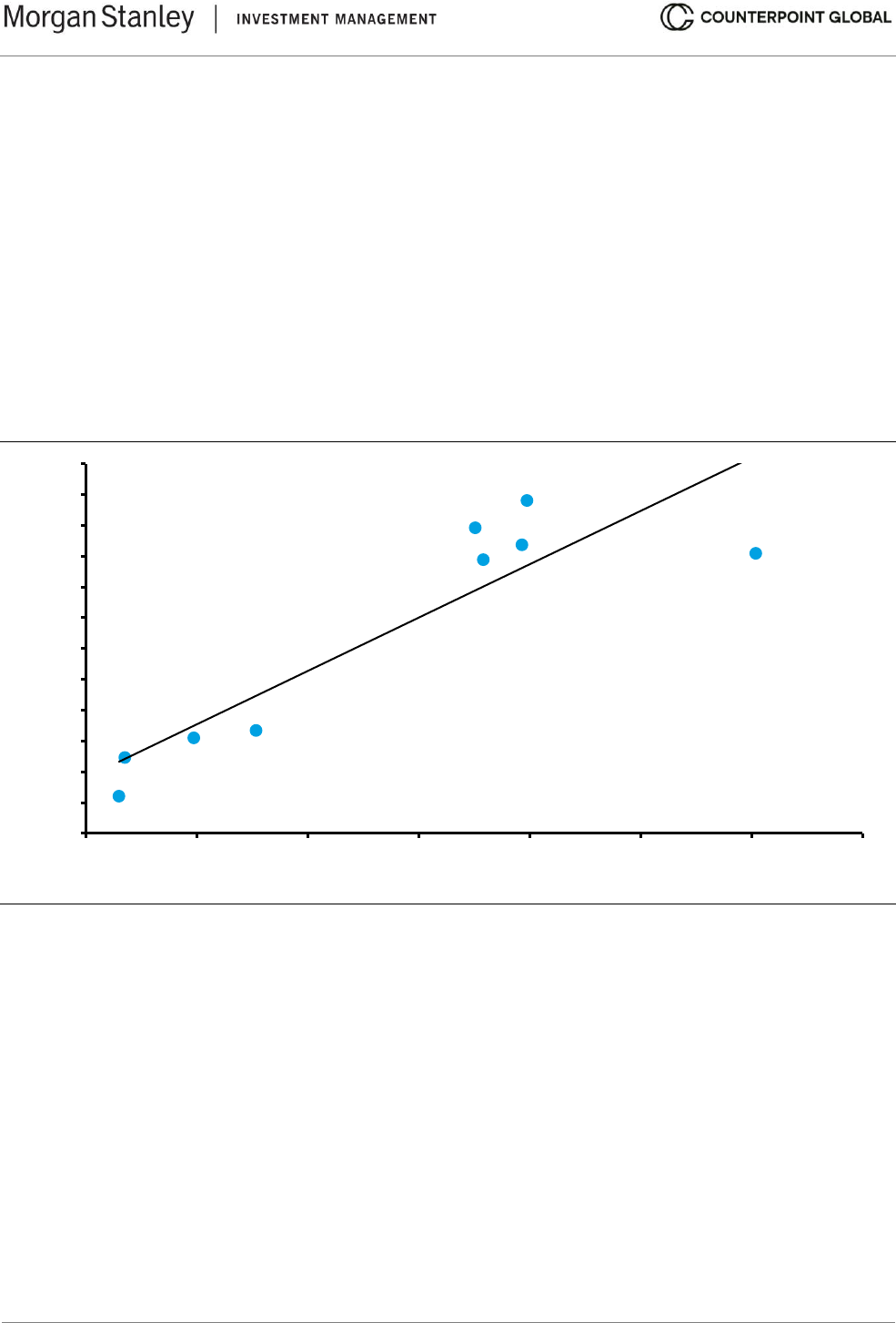
Exhibit 1 shows this relationship over 20 years for 8 asset classes (5 in equities and 3 in credit) and inflation.
Standard deviation, a measure of variation for a set of values, is the proxy for risk, and total shareholder return
(TSR) reflects reward.
Exhibit 1: Risk and Reward for Eight Asset Classes and Inflation, 2003-2022
Source: FactSet; U.S. Bureau of Labor Statistics; Counterpoint Global.
Note: Indexes: MSCI Emerging Markets, Russell 1000, Russell Midcap, Russell 2000, MSCI World, Bloomberg 7-10 Year
U.S. Treasury, Bloomberg U.S. Aggregate Bond, Bloomberg 1-3 Month U.S. Treasury Bills, and U.S. Consumer Price Index.
Portfolio diversification reduces the specific risk of an individual stock, or asset class, but even a portfolio that is
fully diversified is exposed to market risk. What matters for a particular security or asset class is its contribution
to the risk of a diversified portfolio. For instance, the standard deviation of returns for the stock of WD-40
Company, a producer of oil for lubrication, is much higher than that of the market, but adding the stock to a
portfolio reduces risk because the stock tends to zig when the market zags.
8
The focus is not on the risk of the
stock but rather how that security affects the risk of the overall portfolio.
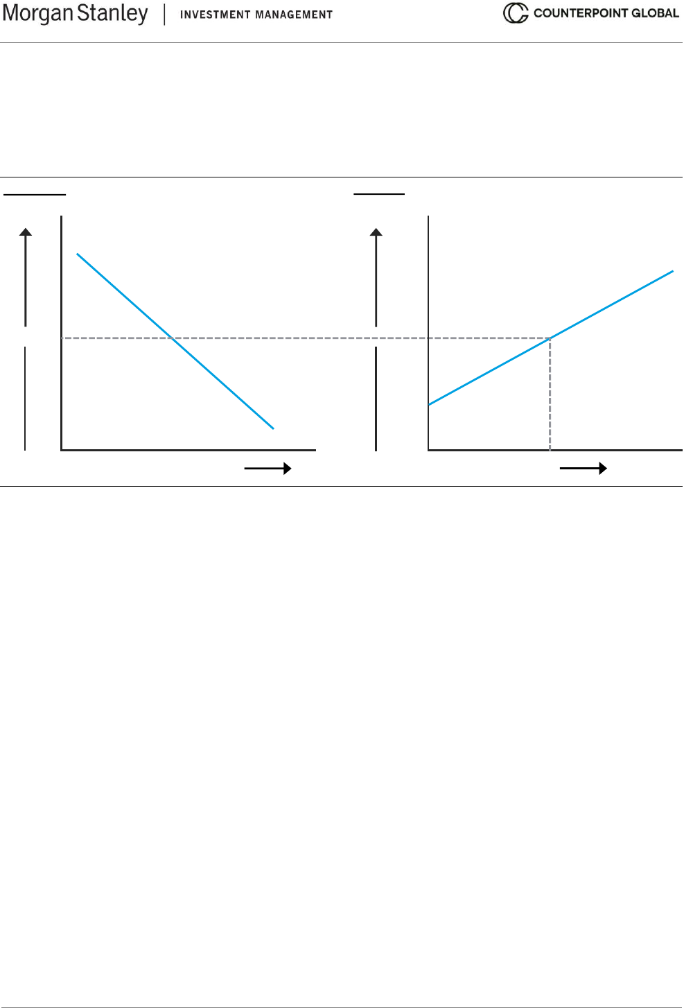
The cost of capital is a link between corporate finance and investing (see exhibit 2). Companies use the capital
that investors save. Companies seek to invest capital, which includes funds generated by the business, at a rate
of return above the cost of capital in order to create value. These capital allocation decisions apply to mergers
and acquisitions (M&A), internally-generated intangible investments, capital expenditures, and working capital.
9
Companies can only invest so much before the return on investment drops below the cost of capital.
0%
1%
2%
3%
4%
5%
6%
7%
8%
9%
10%
11%
12%
0% 5% 10% 15% 20% 25% 30% 35%
TSR (Annual)
Standard Deviation
© 2024 Morgan Stanley. All rights reserved.
6422586 Exp. 2/28/2025
6
The cost of capital for a company is the opportunity cost of the investor. Investors must evaluate investment
opportunities with an eye toward making sure there is an appropriate reward for the risk they take. Investors
vary in their risk appetites but all seek to earn a proper payoff.
Exhibit 2: The Link between Companies and Capital Markets
Source: Based on G. Bennett Stewart, III, The Quest for Value: A Guide for Senior Managers (New York: HarperCollins,
1991), 83.
A company’s balance sheet has assets on the left and liabilities and equity on the right. Assets are the resources
a company employs to generate cash flows. Liabilities and equity are the way a company finances those
resources. Debt and equity are the most popular forms of financial capital.
Debt is a contractual obligation between a company and its lenders, in which the company pledges to make
timely payments of interest and to return principal at the end of a period that is specified by contract. Equity is
technically a contract between a company and its shareholders that confers limited rights to shareholders, which
include the right to vote, transfer ownership, and collect dividends.
10
Practically, common equity represents a claim on future residual cash flows. The claim is on cash flows after a
company has paid other stakeholders, including creditors (interest and principal), suppliers (accounts payable),
the government (taxes), and employees (wages).
We have so far used the standard deviation of asset price changes as a measure of risk. But you can think of
risk more fundamentally as a combination of business risk and financial risk:
11
Corporate risk = business risk + financial risk
Business risk, or asset risk, reflects the variability of operating cash flows. Operating leverage, which measures
changes in operating profit as the result of changes in sales, is an important determinant of business risk.
12
The
ratio of fixed to variable operating costs helps explain operating leverage, especially in the short run. Firms with
high fixed and low variable costs have more operating leverage than those with low fixed and high variable costs.
Financial risk is determined by the amount of debt a company assumes. The interest expense from debt
effectively adds a fixed cost and makes the earnings more volatile.
Return
Prospective Investments
Corporate
WACC
Reward
Risk
Investor
Risk-
Free
Rate

© 2024 Morgan Stanley. All rights reserved.
6422586 Exp. 2/28/2025
7
To see how this works, consider two companies with $100 in operating profit. The first has no debt, so pre-tax
profit and operating profit are the same. The second has debt that incurs $20 in interest expense, which means
that its pre-tax profit is $80.
Now assume that both companies increase their operating profit to $120. The first company will enjoy a 20
percent increase in pre-tax profit (from $100 to $120), while the second company will realize 25 percent growth
in pre-tax profit (from $80 to $100). Naturally, the math also has a similar effect on the downside. Even with the
same operating income, profits are more volatile for the second company than they are for the first. Empirically,
companies with high business risk tend to have low financial risk, and companies with low business risk benefit
from having some financial risk.
13
Franco Modigliani and Merton Miller (M&M), economists who received the Nobel Memorial Prize in Economic
Sciences, developed a theorem in the late 1950s showing that the value of a firm is independent of its capital
structure.
14
Their point, which ran against the conventional wisdom of the time, was that a change in the capital
structure does not change risk overall but rather simply transfers risk from one stakeholder to another.
The cost of debt also goes up when a company adds debt because the size of the contractual obligation grows.
The cost of equity also goes up because the magnitude of the senior claims on assets is higher, making the
return on the residual claim riskier. But overall risk is preserved since debt is less costly than equity due to its
seniority in the capital structure.
A simple illustration can help make the point. Assume a company that has $100 in annual operating profit. We
can observe what happens as we add debt to the capital structure.
A B C
Operating profit $100 $100 $100
Debt 0 200 400
Cost of debt 0.00% 5.00% 6.25%
Cash flow for equity 100 90 75
Equity 1,000 800 600
Cost of equity 10.00% 11.25% 12.50%
Value of the firm $1,000 $1,000 $1,000
In scenario A, the firm is financed solely with equity that has a cost of 10 percent. Provided the company will
earn $100 into perpetuity with no growth, the value of the firm is $100 divided by 10 percent, or $1,000.
In scenario B, the company issues $200 of debt at a cost of 5 percent. As a result, the cash flow for equity
holders drops $10, from $100 to $90 ($10 = $200 × 5 percent). Shareholders now require a return of 11.25
percent because the addition of debt increases their risk. The debt is $200, the equity is now worth $800 ($800
= $90 ÷ 11.25 percent), and the value of the firm remains $1,000 ($1,000 = $200 debt + $800 equity).
In scenario C, the company adds more debt, bringing the total to $400. The additional debt increases the risk
for debt holders. As a consequence, the cost of debt goes from 5 to 6.25 percent. The higher interest payment,
now $25 ($25 = $400 × 6.25 percent), means that only $75 is left over for equity holders. The risk for equity
holders also rises, going from 11.25 to 12.5 percent. Here again, the cost of debt and equity are higher but the
value of the firm does not change. The debt is worth $400 and the equity is valued at $600 ($600 = $75 ÷ 12.5
percent), leaving the total at $1,000.

© 2024 Morgan Stanley. All rights reserved.
6422586 Exp. 2/28/2025
8
M&M’s invariance proposition offers insight because it is true only under very specific conditions, including no
taxes, bankruptcy costs, or effects on managerial incentives. It also assumes markets are perfect and complete.
Since none of these conditions prevail in the real world, we can conclude capital structure does matter.
15
To see why, we focus on the assumption of no taxes. Many tax codes, including that of the U.S., treat some
percentage of interest expense as a deduction from income before paying taxes. That means some debt adds
value to the firm up to a point because more cash flow is going to stakeholders and less is going to the
government.
Debt’s impact on the cost of capital is based on the role of taxes and other factors rather than on how a company
slices and dices its capital structure. Further, too much debt is problematic because it introduces the risk of
financial distress.
We are about to roll up our sleeves and get into the details. But to summarize, the cost of capital is the opportunity
cost of the investors who provide capital. It serves as a crucial link between corporate finance and investing, as
it sets the minimum rate of return a company should be willing to accept to invest in its business.
Risk can be disaggregated into business risk, which reflects the volatility of a firm’s cash flows, and financial
risk, how much debt the company takes on. M&M shows that capital structure does not matter under conditions
that are unrealistic. When we introduce realistic conditions, we can see that capital structure does matter and
that it affects the cost of capital.
Some investors prefer to discount cash flows at a required rate of return that reflects the minimum threshold of
expected return they want to earn. In cases when that rate of return exceeds the cost of capital, the approach is
equivalent to discounting at the cost of capital and insisting on paying a price that is sufficiently less than value.

© 2024 Morgan Stanley. All rights reserved.
6422586 Exp. 2/28/2025
9
Estimating the Cost of Debt
The cost of debt is the effective after-tax rate a company has to pay on its long-term debt.
The yield to maturity on a company’s long-term, option-free bonds is a good estimate for the pre-tax cost of debt
for a company with securities that are rated as investment grade. This is debt that is deemed to have a relatively
low risk of default and hence receives a higher rating from the credit agencies (Baa or above from Moody’s and
BBB or above from S&P Global and Fitch). You can observe this rate directly for most firms.
For companies that have only short-term or illiquid debt, you can take some steps to estimate the cost of debt
indirectly. First, determine the credit rating on the company’s unsecured long-term debt. Second, look at the
average yield to maturity on a portfolio of bonds with a similar credit rating. Bond investors often express this as
a spread over a Treasury rate, usually the 10-year note. The treasury yield is a proxy for the risk-free rate.
It is appropriate to use an option-adjusted spread (OAS) for a fixed income security that embeds options. For
example, a bond may include an option for the investor to sell it back to the issuer on a specific date at a set
price. Or the issuer may have the option to call back, or redeem, the bond at a predetermined time and price.
Some companies finance themselves predominantly with short-term debt. In this case, it may appear appropriate
to use the short-term rates as the cost of debt, but the problem is that short-term rates do not reflect expectations
about long-term inflation. The time horizon for estimating the cost of capital should match the time horizon of
forecasted cash flows, which is rarely less than ten years.
The long-term rate is a better approximation of interest costs over time even for companies that roll over their
short-term debt because long-term rates capture the expected cost of repeated borrowing. If a company
exclusively relies on short-term debt, use its credit rating to approximate the cost of long-term debt.
Free cash flow, or net operating profit after taxes (NOPAT) less investment needs, does not reflect financial
leverage. This is useful for comparing companies with different capital structures. But debt creates a valuable
tax shield free cash flow does not capture because some of the interest expense is generally tax deductible.
16
To capture the value of the tax shield, you must adjust debt from a pre-tax rate to an after-tax rate. To do this,
multiply the pre-tax cost of debt by one minus the marginal tax rate. The marginal tax rate is the tax rate a
company pays on its last dollar of taxable income. This is how the benefit of the tax shield that debt creates finds
its way into the calculation of WACC. The formula is:
After-tax cost of debt = pre-tax cost of debt × (1 – marginal tax rate)
Not all companies can take all of their interest expense as a deduction from taxes. For example, the Tax Cuts
and Jobs Act of 2017 sets a limit on the tax deductibility of interest at 30 percent of earnings before interest and
taxes (EBIT) for U.S. companies with sales of $25 million or more. This went into effect in 2022. We estimate
that this affected about 25 percent of the companies in the Russell 3000 that had positive EBIT in 2022. The
Russell 3000 tracks the largest stocks by market capitalization in the United States.
The effective rate is commonly lower than the marginal rate because companies have net operating losses
(NOLs), tax loss carrybacks, or investment tax credits.
The cost of debt should reflect the marginal rate, including state and local taxes, of the countries where the
company earns its operating profit. This can create a sizeable difference between the tax rate in a company’s
home country and the tax rate it must actually pay for firms with a large presence outside of their domicile.
© 2024 Morgan Stanley. All rights reserved.
6422586 Exp. 2/28/2025
10
For companies with tax loss carryforwards, it may make sense to value the company in two stages. First, assume
the company pays normal taxes in its free cash flows. This, of course, will lead to a value that is too low.
Second, calculate the present value of the tax savings. To do this, calculate the annual tax savings and discount
that savings at the cost of debt. Note that the company has to produce operating income to realize tax savings.
Add that amount back to the value of the firm assuming full tax payment. These two stages allow for
comparability to profitable peers and specify the value of the tax savings.
The Tax Cuts and Jobs Act of 2017 also changed the rules for NOLs. Prior to the act, companies could carry
back NOLs for two years, carry them forward for 20 years, and offset all taxable income when carried back or
forward. Starting in 2018, carrybacks were eliminated and companies are only allowed to use a net operating
loss carryforward for up to 80 percent of taxable income.
The book value of debt is in many cases a sensible proxy for the market value of debt. But make an adjustment
in your debt-to-total capital ratio if the debt is trading at a substantial premium or discount to par.
The yield to maturity is a reasonable proxy for the pre-tax cost of debt for companies with debt that is rated as
investment grade. That yield can be expressed as a spread over a risk-free rate.
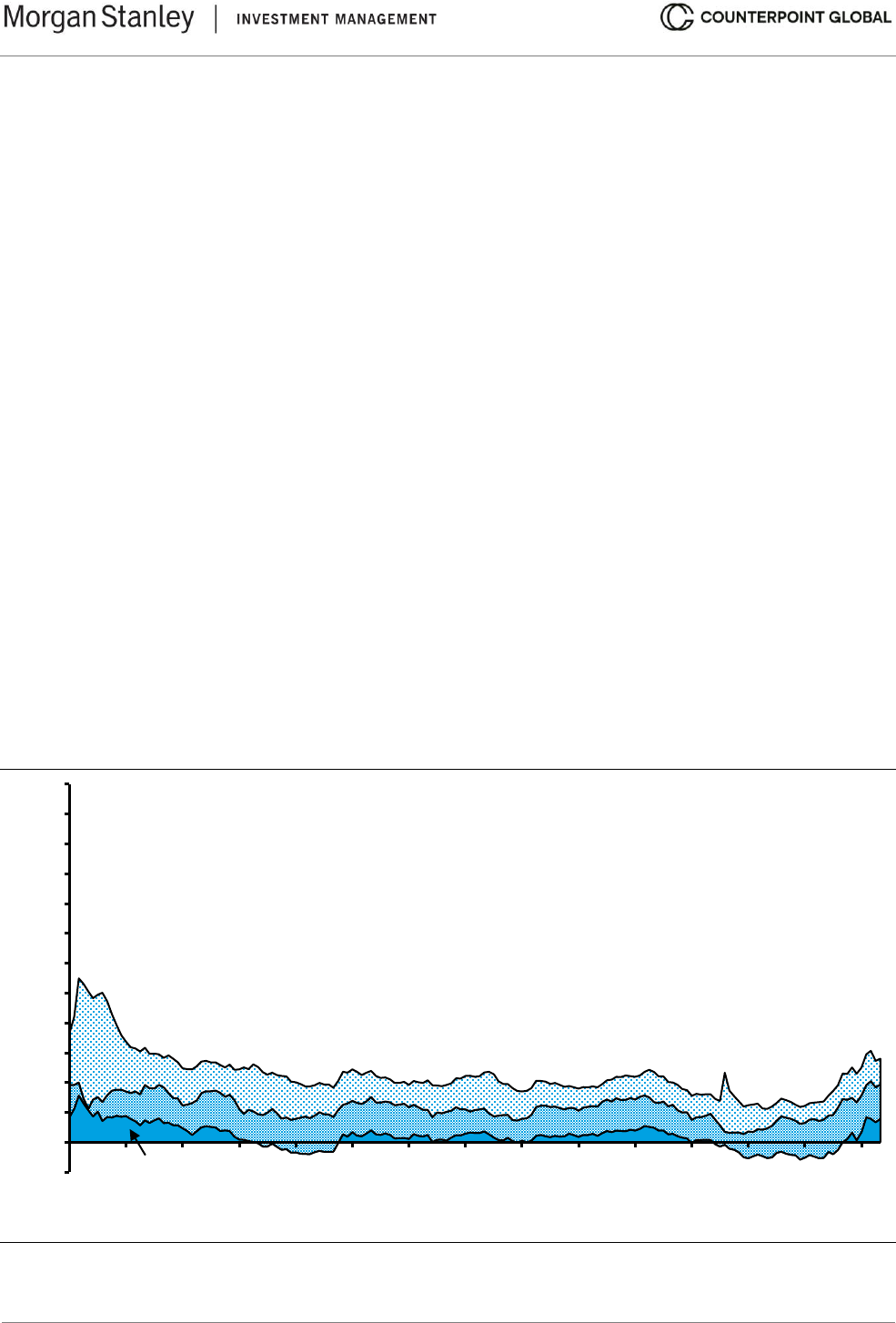
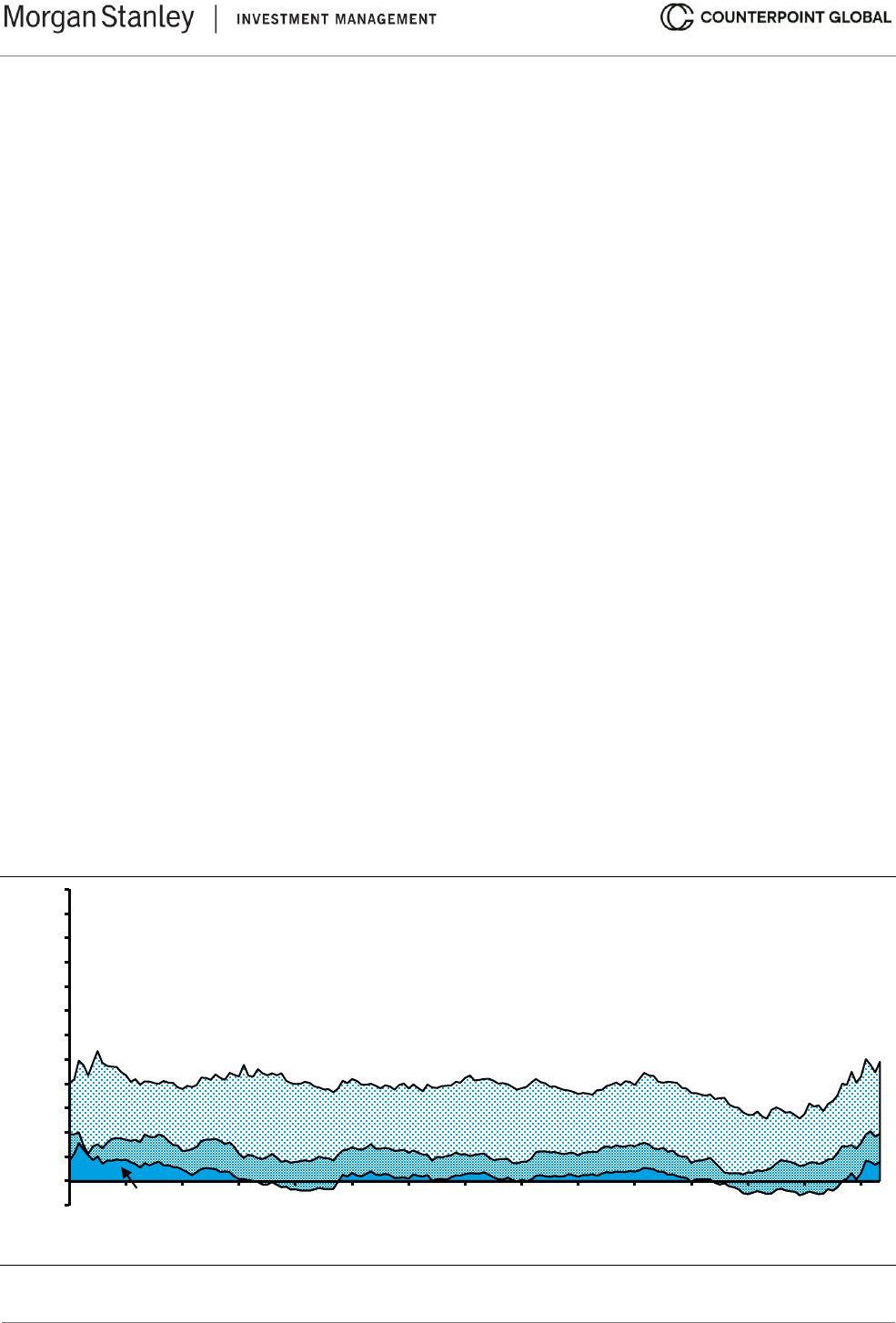
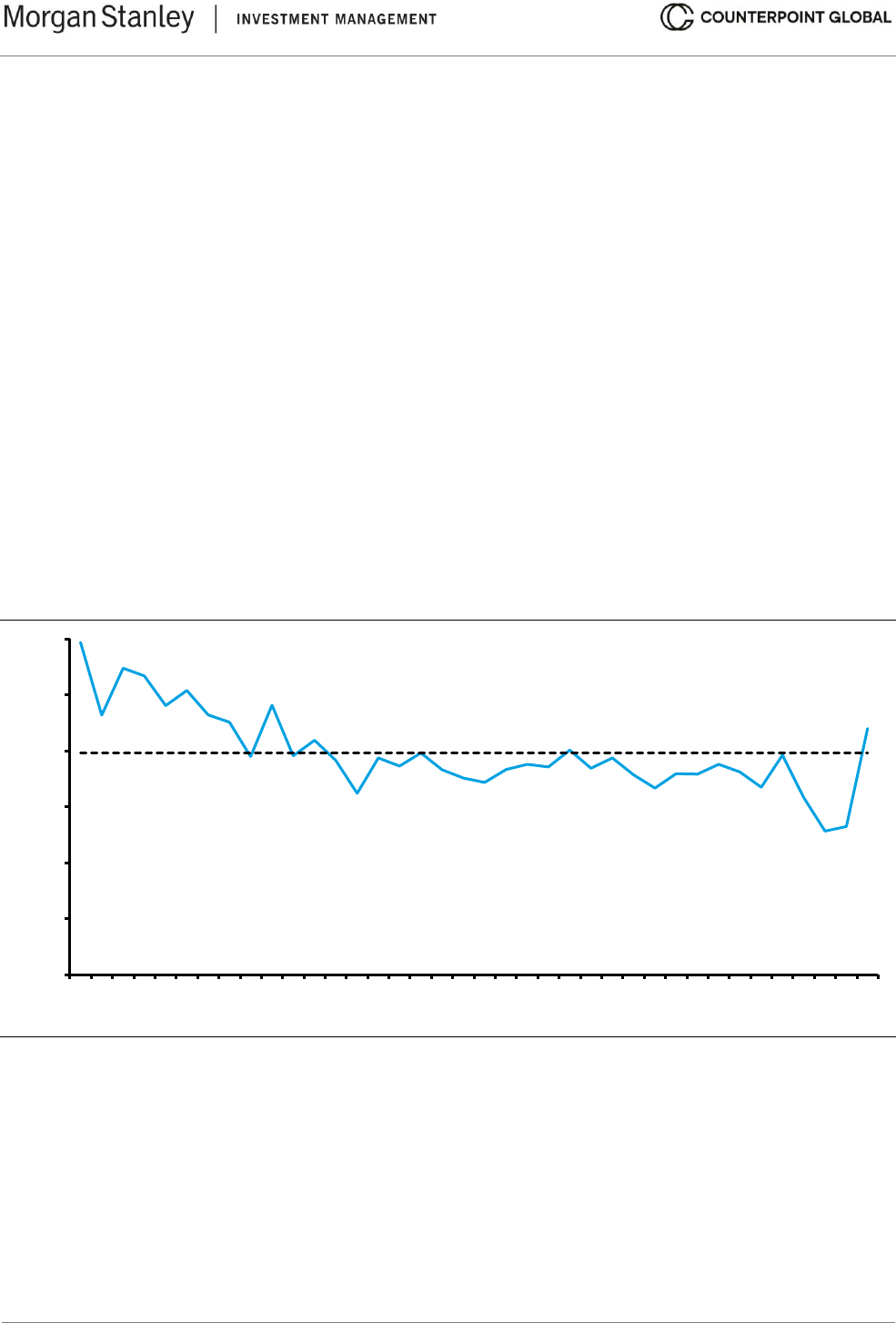
Exhibit 3 shows a decomposition of expected returns, calculated monthly, for BBB bonds from 2008 to 2022.
The components of the expected return include the real yield on the 10-year U.S. Treasury note, inflation
expectations, and the BBB credit spread. The nominal yield on the 10-year U.S. Treasury note equals the real
yield plus inflation expectations.
Over this time, the spread peaked at 7.8 percentage points in December 2008 during the financial crisis and
troughed at 1.1 percentage points in June 2021 in the throes of COVID.
Exhibit 3: Expected Returns on BBB Bonds Calculated Monthly, 2008-2022
Source: Aswath Damodaran; FRED at the Federal Reserve Bank of St. Louis; Counterpoint Global.
Note: August 2008-December 2022; Treasury note=10-year U.S. Treasury note; BBB spread=ICE BofA BBB U.S. corporate
index option-adjusted spread.
-2
0
2
4
6
8
10
12
14
16
18
20
22
24
2008
2009
2010
2011
2012
2013
2014
2015
2016
2017
2018
2019
2020
2021
2022
Percent
BBB Credit Spread
Inflation Expectations
Treasury Note Real Yield
© 2024 Morgan Stanley. All rights reserved.
6422586 Exp. 2/28/2025
11
Yield to maturity overstates the pre-tax cost of debt for companies issuing high-yield debt, or debt that is rated
below investment grade.
17
The reason is that high-yield bonds have a meaningful probability of default. For
example, the base rate of default over 10 years is about 2 percent for an investment-grade bond (BBB- or higher)
and 23 percent for a speculative-grade bond (BB+ or lower).
18
The following equation is relevant for all bonds:
Cost of debt = promised yield spread – lost yield due to default
The cost of debt is somewhere between the promised yield and the risk-free rate. Because the lost yield due to
default is negligible for companies that issue investment-grade bonds, the cost of debt and promised yield are
practically equivalent. That means the yield to maturity is a suitable proxy for the cost of debt for companies that
issue investment-grade bonds.
The lost yield due to default can be consequential for companies with non-investment grade ratings. As a
consequence, that yield to maturity may overstate materially the cost of debt. We will describe how to estimate
the lost yield due to default in a moment.
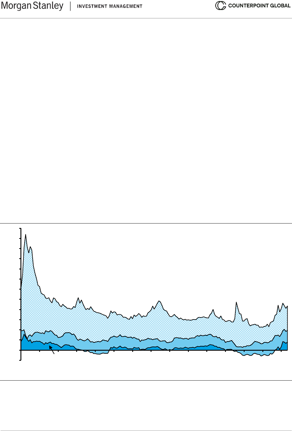
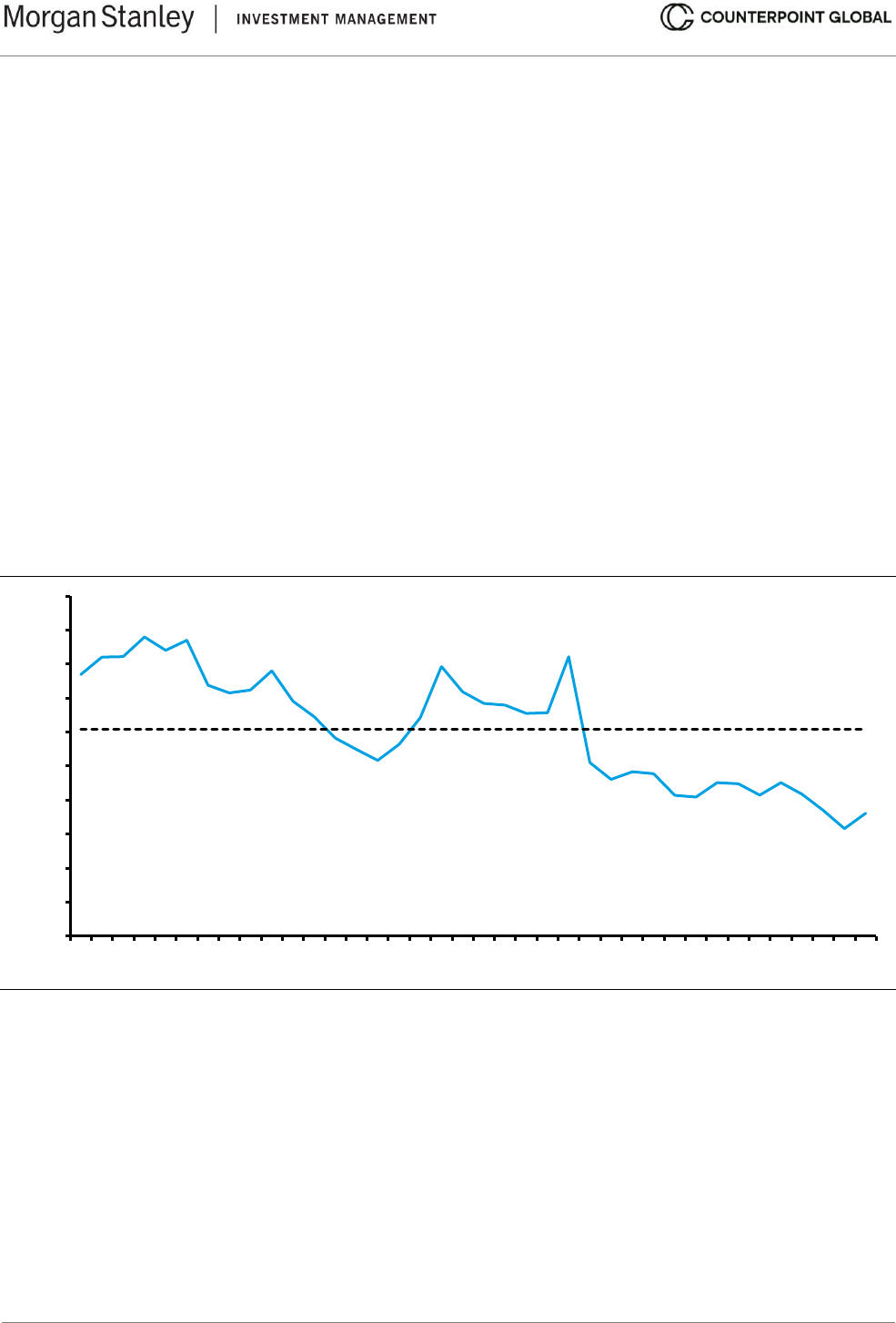
Exhibit 4 shows a decomposition of expected returns, calculated monthly, for high-yield bonds from 2008 to
2022. The spread peaked at 19.9 percentage points in November 2008, implying an expected return in excess
of 20 percent, near the climax of the financial crisis. It bottomed at 3.0 percentage points, or an expected return
of 4.5 percent, in June 2021 during COVID.
Exhibit 4: Expected Returns on High Yield Bonds Calculated Monthly, 2008-2022
Source: Aswath Damodaran; FRED at the Federal Reserve Bank of St. Louis; Counterpoint Global.
Note: August 2008-December 2022; Treasury note=10-year U.S. Treasury note; High yield spread=ICE BofA U.S. high-yield
index option-adjusted spread.
-2
0
2
4
6
8
10
12
14
16
18
20
22
24
2008
2009
2010
2011
2012
2013
2014
2015
2016
2017
2018
2019
2020
2021
2022
Percent
High Yield Credit Spread
Inflation Expectations
Treasury Note Real Yield

© 2024 Morgan Stanley. All rights reserved.
6422586 Exp. 2/28/2025
12
Robert Merton, a professor of finance who was also accorded the Nobel Memorial Prize in Economic Sciences,
developed a model that can provide insight into the risk of lost yield due to default.
19
The model values the equity
value of a company as a call option on its assets with a strike price equivalent to the notional value of the
liabilities. The key is that the distribution of option values provides insight into the default probability.
Ian Cooper and Sergei Davydenko, professors of finance, use the Merton model to estimate the lost yield due
to default. Their inputs include the debt-to-total capital ratio, credit spread, equity risk premium, and volatility of
the equity. They estimate, for example, that the proportion of the debt spread attributable to lost yield due to
default is 13 basis points, or 13 percent of the spread, for a firm with a 20 percent debt-to-total capital ratio, a
100 basis point credit spread over AAA-rated bonds, an equity risk premium of 6 percent, and a volatility of
equity of 30 percent. Accordingly, using the expected return results in a small error.
The picture is very different for a firm with high leverage. Assume a company has a 70 percent debt-to-total
capital ratio, a 400 basis point credit spread of AAA-rated bonds, an equity risk premium of 6 percent, and a
volatility of equity of 50 percent. The debt spread attributable to lost yield due to default rises to nearly 250 basis
points, or 62 percent of the spread. In this case, the promised yield spread greatly overstates the cost of debt.
Leases should also be considered debt. In 2019, new guidelines from the Financial Accounting Standards Board
(FASB), which establishes U.S. Generally Accepted Accounting Principles (GAAP), required most companies
to reflect leases longer than one year on the balance sheet.
20
Leases appear as a right-of-use asset on the asset
side of the balance sheet. This captures the lessee’s right to use the asset over the duration of the lease. About
three trillion dollars of leases were added to the balance sheets of U.S. companies as a result of this accounting
change.
21
In a quirk of accounting under GAAP, the entire lease payment, including embedded interest, is reflected in the
calculation of EBIT. With debt, the interest expense shows up below EBIT. As a result, a company that leases
an asset will have lower EBIT than a company that finances the asset with debt, even though pre-tax income
will be the same. By contrast, lease payments are appropriately allocated between depreciation and interest
expense under International Financial Reporting Standards (IFRS).
Total net debt should include leases and unfunded retirement benefits minus excess cash. Depending on the
business, you can treat cash and marketable securities above two to five percent of sales as excess.
For example, Amazon, a multinational technology company, had long-term lease liabilities of $73.0 billion as of
December 31, 2022. This liability was comprised of $11.4 billion in capital leases and $61.6 billion in operating
leases. Total debt was $70.1 billion, including short-term debt of $3.0 billion and long-term debt of $67.1 billion.
Total lease liabilities plus debt equaled $143.1 billion.
The combination of cash and marketable securities was $70.0 billion, and sales for 2022 were $514 billion.
Assuming the company requires 2 percent of sales to operate, excess cash was $59.7 billion ($59.7 = $70.0 –
[$514 × .02]). Total net debt was $83.4 billion ($83.4 = $73.0 in leases + $70.1 in debt - $59.7 in excess cash).
The company’s equity value on that date was $860 billion ($860 = $84.00 stock price × 10.2 billion shares
outstanding).
Estimating the cost of debt is a reasonably straightforward process for most companies. The calculation is more
challenging for companies that have debt that is rated below investment grade or substantial leases or other
liabilities.

© 2024 Morgan Stanley. All rights reserved.
6422586 Exp. 2/28/2025
13
Estimating the Cost of Equity
The cost of equity is the expected total return on a company’s stock.
The cost of equity is higher than the cost of debt because equity is a junior claim on the value of a firm. In
addition, debt is an even cheaper source of financing because some percentage of the interest expense on debt
is tax deductible. An estimate of the cost of equity should never be lower than that of debt.
The cost of equity is difficult to estimate because we cannot observe it directly. For example, when a company
issues debt the cost is relatively transparent. The same company offering equity can only approximate the cost.
As a consequence, an estimate of the cost of equity requires an asset-pricing model.
The best known of these are the capital asset pricing model (CAPM), developed by a handful of economists,
including William Sharpe, and the three-factor model, advanced by Eugene Fama and Kenneth French,
professors of finance.
22
Sharpe and Fama were also awarded the Nobel Memorial Prize in Economic Sciences.
Academics have continued to add factors in an effort to explain returns more effectively than the CAPM or three-
factor model can. This has led to a “zoo” of factors seeking to explain hundreds of purported anomalies.
23
Financial executives rely heavily on the CAPM but the investment community, led by quantitative funds, uses
six factors widely. These include beta (stocks of companies with high betas earn higher returns than those with
low betas), size (stocks of companies with small capitalizations generate higher returns than stocks of
companies with large capitalizations),
24
value (stocks with low multiples outperform those with high multiples),
25
momentum (stocks that have done well continue to do well in the short term),
26
quality (companies of high quality
provide higher returns than companies of low quality),
27
and asset growth (companies with low asset growth
outperform those with high asset growth).
28
Fama and French now recommend a five-factor model that includes all of the factors above except for
momentum. We will focus on the CAPM because it is the model most practitioners use. See appendix B for a
discussion of the three-factor model.
The CAPM estimates the expected return of a security by adding the risk-free rate to the security’s beta (β) times
the equity risk premium (ERP). The ERP equals the difference between the expected return for the market and
the risk-free rate and is similar conceptually to a credit spread.
Expected return = Risk-free rate + β(Market return – Risk-free rate)
The ERP is the same for all stocks in the CAPM because it captures what is known as “systematic risk,” or risk
that cannot be diversified away. Beta measures how a company’s risk contributes to portfolio risk. “Unsystematic
risk” can be reduced through portfolio diversification.
Exhibit 5 shows the security market line, which reflects a linear relationship between risk and reward. Beta
measures how much a stock moves relative to a benchmark index.

© 2024 Morgan Stanley. All rights reserved.
6422586 Exp. 2/28/2025
14
Exhibit 5: The Security Market Line
Source: Counterpoint Global.
The CAPM was developed in the early 1960s, and empirical tests of the model made it clear pretty early on that
it is better in theory than in practice. Even before introducing additional factors, practitioners have to use
judgment to answer questions about three of the model’s key drivers:
• What is the appropriate risk-free rate?
• How should the equity risk premium be estimated?
• What is the best method to estimate beta?
Risk-Free Rate. The best proxy for the risk-free rate is a yield on a long-term, default-free government fixed-
income security. The yield on the 10-year U.S. Treasury note is appropriate for businesses based in the United
States. This yield is easy to find, is sufficiently long-dated, and has a relatively low risk of default.
Outside of the United States, you can adjust the government borrowing rate in local currencies by the estimated
default spread. Aswath Damodaran, a professor of finance at the Stern School of Business at New York
University, shares these estimates on his website based on local currency ratings.
29
Ideally, the security that reflects the risk-free rate should have no covariance with the market, or a beta of zero.
Exhibit 6 shows that the 10-year Treasury note has a beta of 0.03 when compared to the S&P 500, an index
that tracks the stocks of 500 large companies in the U.S. These are monthly returns for the 60 months ending
in December 2022.
Security Market Line (SML)
Rate of Return
Risk (Beta Coefficient)
Risk-
Free
Rate
© 2024 Morgan Stanley. All rights reserved.
6422586 Exp. 2/28/2025
15
Exhibit 6: Beta for 10-Year U.S. Treasury Note versus the S&P 500, 2018 to 2022
Source: FactSet and Counterpoint Global.
Note: Returns for 10-Year Note represented by the Bloomberg U.S. Treasury 7-10 Year TR Index.
Equity Risk Premium. The ERP is the difference between the return of the equity market and the return of the
risk-free asset.
30
The ERP is higher than credit spreads in general because equity is riskier than debt. Observing
the historical ERP is easy but estimating the premium going forward is a challenge. For example, one survey of
150 finance and valuation textbooks that were written over 3 decades revealed a range of estimated ERPs from
3 to 10 percent, and one-third of the books used different ERPs in various places within the same book.
31
Leading academics and practitioners who convened a meeting in 2001 to discuss the ERP provided a range of
estimates for the ERP at that time from 0 to 7 percent, with an average just under 4 percent.
32
The realized ERP
for the following 10 years was minus 4.1 percent.
Determinants of the ERP include collective risk aversion, the perceived level of economic risk, the degree of
liquidity in markets, and tax policy.
33
The ERP moves around because these factors change. In fact, academic
research suggests the ERP is probably a series that has unstable statistical properties.
34
The practical objective
is to come up with an intelligent forecast of the ERP to assess expected returns.
There are three common approaches to estimating the ERP. The first is to look at historical results and assume
the future will be similar to the past. The second is to survey investors about their expectations. The third is to
estimate a rate the market implies by reverse-engineering assumptions to solve for the market price.
Each approach has its pros and cons. Historical results are supported by lots of data but are highly sensitive to
the time period selected, include survivorship bias, and are different whether calculated using arithmetic or
geometric averages.
35
Surveys, which include forecasts by academics, financial executives, and individual and institutional investors,
provide snapshots of attitudes at a specific moment but are imperfect because of a strong tendency to
extrapolate recent results. The structures of the surveys are not always ideal.
36
-5
-4
-3
-2
-1
0
1
2
3
4
5
-15 -10 -5 0 5 10 15
10-Year Note Monthly Returns (Percent)
S&P 500 Monthly Returns (Percent)
Slope = 0.03

© 2024 Morgan Stanley. All rights reserved.
6422586 Exp. 2/28/2025
16
An ERP implied by the market uses current prices but requires forecasts for drivers such as cash flow growth
and return on capital. Aswath Damodaran posts an updated estimate of the equity risk premium on his website
every month. He also shares a spreadsheet with his assumptions that offers the flexibility to change the variables.
Damodaran has annual estimates for the equity risk premium going back to 1961. The range is from a low of 2.1
percent in 1999 to a high of 6.5 percent in 1979. The estimates are not adjusted for inflation.
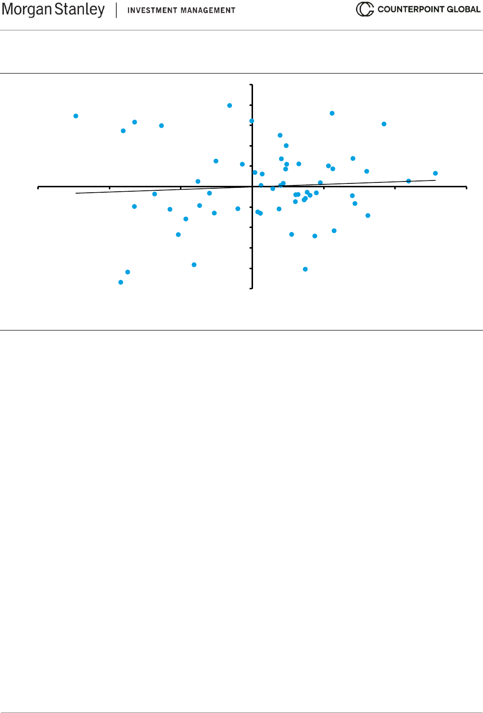
Exhibit 7 shows the relationship between Damodaran’s cost of equity estimates (x-axis) and the subsequent
total returns for the S&P 500 over the following 10 years (y-axis). While not perfect, there is a distinct association
between expected and realized returns.
We find Damodaran’s estimates to be sensible and note that FactSet uses his equity risk premium as the default
in their calculations of the cost of capital.
Exhibit 7: Cost of Equity and Future TSRs, S&P 500, 1961-2022
Source: FactSet; Aswath Damodaran; Counterpoint Global.
We ultimately want an ERP that looks forward, but understanding historical averages is helpful to place current
conditions in context. Calculating the historical ERP might appear straightforward, but it requires judgment about
the appropriate risk-free rate, the time period over which to measure results, and the choice of an arithmetic or
geometric average. Damodaran finds that the historical ERP can fall in the range of 3 to 12 percent based on
the various combinations of alternatives.
37
The total return on the 10-year Treasury note works well as a proxy for the risk-free rate. Using returns from
Treasury bills or bonds requires a commensurate adjustment to the ERP.
The issue of time horizon is thornier. The argument in favor of shorter time horizons is that they better capture
present conditions. The argument against a short time frame is that it may not accurately reflect the full
distribution of outcomes. An estimate’s accuracy can be measured with the standard error, which is calculated
as the observed standard deviation divided by the square root of the sample size.
In plain words, using a small sample of a large distribution of outcomes increases the possibility that your
estimate is wrong because you fail to capture a lot of relevant data. For example, returns for the S&P 500 since
-2%
0%
2%
4%
6%
8%
10%
12%
14%
16%
18%
20%
0% 2% 4% 6% 8% 10% 12% 14% 16% 18% 20%
S&P 500 TSR,
Next 10 Years (Annualized)
Cost of Equity
r = 0.66
© 2024 Morgan Stanley. All rights reserved.
6422586 Exp. 2/28/2025
17
1928 have had a standard deviation of just under 20 percent. That series includes more than 90 years, which
gets the standard error down to about 2.0 percent (0.02 = 0.197 ÷ 94^
0.5
). That the standard errors are as large
or larger than the ERP for periods of fewer than 20 years supports the case for a longer time period.
Historical averages to estimate the ERP can be calculated using arithmetic or geometric returns. The difference
between the two is material. The arithmetic mean is the average of the annual ERPs (equity market - risk-free
rate). The geometric mean is the compound annual rate of return. The geometric return is always less than or
equal to the arithmetic return and can be approximated by taking one-half of the variance of returns. Variance is
the square of the standard deviation.
The difference between arithmetic and geometric returns grows as the standard deviation of the results in the
time series increases. For equity less bond returns in the U.S. from 1928-2022, the arithmetic return was 6.6
percent and the geometric mean was 5.1 percent. The difference, 1.5 percentage points, is a large percentage
of the value of both totals.
The arithmetic average is appropriate if the objective is to estimate the equity risk premium over the next year.
The geometric average is proper over multiple time periods.
The second approach is an estimate of the ERP implied by market prices. The idea is that the key drivers of
value, including earnings and dividends, follow long-term trends that are somewhat predictable. With a sense of
future cash flows and knowledge of the prevailing price, it is possible to solve for the discount rate that equates
the present value of future free cash flows to today’s price.
Exhibit 8 shows the expected returns for the U.S. stock market from August 2008 through 2022 using the 10-
year Treasury note as the risk-free rate and Damodaran’s estimate of the ERP. The average ERP over this
period was 5.5 percent, with a high of 7.7 percent in February 2009 and a low of 3.9 percent in July 2021.
Expected return, which adds the yield on the 10-year U.S. Treasury note to the ERP, peaked at 10.7 percent in
February 2009 and bottomed at 5.1 percent in December 2020. All of these figures are unadjusted for inflation.
In 2022, expected returns jumped from 5.8 percent at the beginning of the year to 9.8 percent at the end.
Exhibit 8: Expected Return on U.S. Equities Calculated Monthly, 2008-2022
Source: Aswath Damodaran; FRED at the Federal Reserve Bank of St. Louis; Counterpoint Global.
Note: August 2008-December 2022; Treasury note=10-year U.S. Treasury note.
-2
0
2
4
6
8
10
12
14
16
18
20
22
24
2008
2009
2010
2011
2012
2013
2014
2015
2016
2017
2018
2019
2020
2021
2022
Percent
Equity Risk Premium
Inflation Expectations
Treasury Note Real Yield
© 2024 Morgan Stanley. All rights reserved.
6422586 Exp. 2/28/2025
18
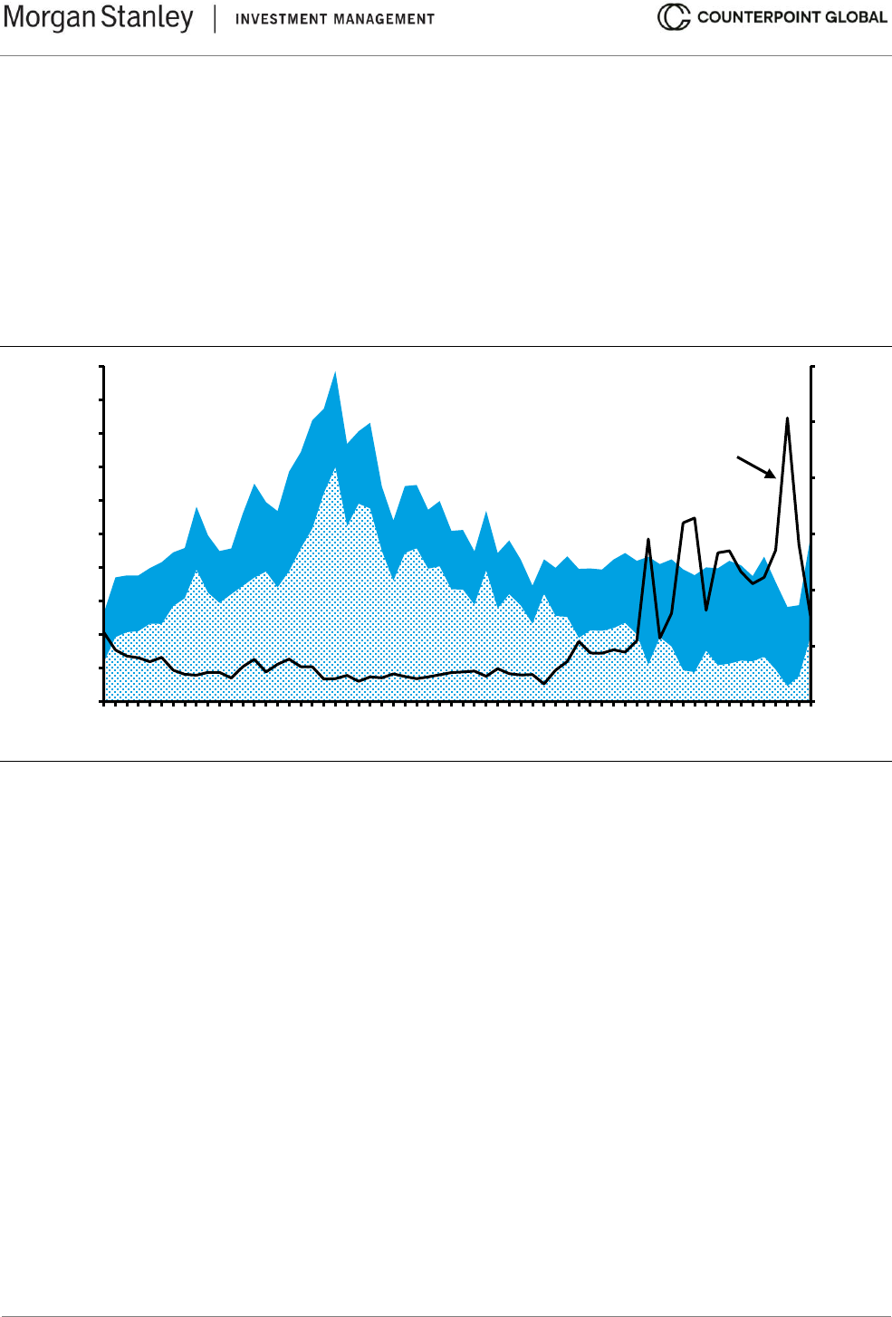
Exhibit 9 shows the risk-free rate, the implied ERP, and the ratio between the two from 1961 to 2022. This
provides a sense of the sources of return. From 1961 through about 2000, the ratio of the ERP to the risk-free
yield was about 0.6, which means that the ERP was consistently below the risk-free rate.
That ratio started rising following the dot-com bust, jumped after the financial crisis, and spiked to more than five
times with the actions taken to deal with COVID. In 2022, the estimated ERP increased 170 basis points and
the yield on the risk-free rate rose 230 basis points, lowering the ratio between the ERP and risk-free rate to
about 1.5 times. The current ratio is in line with those in the 2000s, while still far from the average of 1961-1999.
Exhibit 9: Equity Risk Premium and the Risk-Free Rate, 1961-2022
Source: Aswath Damodaran; FRED at the Federal Reserve Bank of St. Louis; Counterpoint Global.
Note: Data reflect end of year; Treasury note=10-year U.S. Treasury note.
Comparing the ERP to credit spreads is another way to assess whether it is calibrated sensibly. We can use
expected fixed income returns, which are observable, as a benchmark to estimate expected equity returns,
which are unobservable.
The ERP is higher than the credit spread because stocks are riskier than bonds. However, there have been
periods of very high valuations in the equity markets that implied low future equity returns. The peak of the
market in March 2000 is an example.
38
Returns for large-capitalization stocks were poor for the following decade
relative to history.
Exhibit 10 shows the relationship between the ERP and the spread between bonds rated Baa by Moody’s and
the risk-free rate from 1980 through 2022. On average, the ERP has averaged around 2.0 times the credit
spread. A ratio above the average suggests that stocks are attractive relative to investment-grade bonds, and a
ratio below the average implies that bonds look good relative to stocks. The ratio was 3.0 at the end of 2022.
0
1
2
3
4
5
6
0%
2%
4%
6%
8%
10%
12%
14%
16%
18%
20%
1961
1964
1967
1970
1973
1976
1979
1982
1985
1988
1991
1994
1997
2000
2003
2006
2009
2012
2015
2018
2021
Equity Risk Premium /
Treasury Note Yield
Equity Risk Premium and
Treasury Note Yield
ERP /
Treasury
Note Yield
Equity Risk
Premium
Treasury
Note Yield
© 2024 Morgan Stanley. All rights reserved.
6422586 Exp. 2/28/2025
19
Exhibit 10: Equity Risk Premium and Baa Spread, 1980-2022
Source: Aswath Damodaran; FRED at the Federal Reserve Bank of St. Louis; Counterpoint Global.
Note: Data reflect end of year; Baa spread=Moody's Seasoned Baa Corporate Bond Yield minus yield on 10-year U.S.
Treasury note.
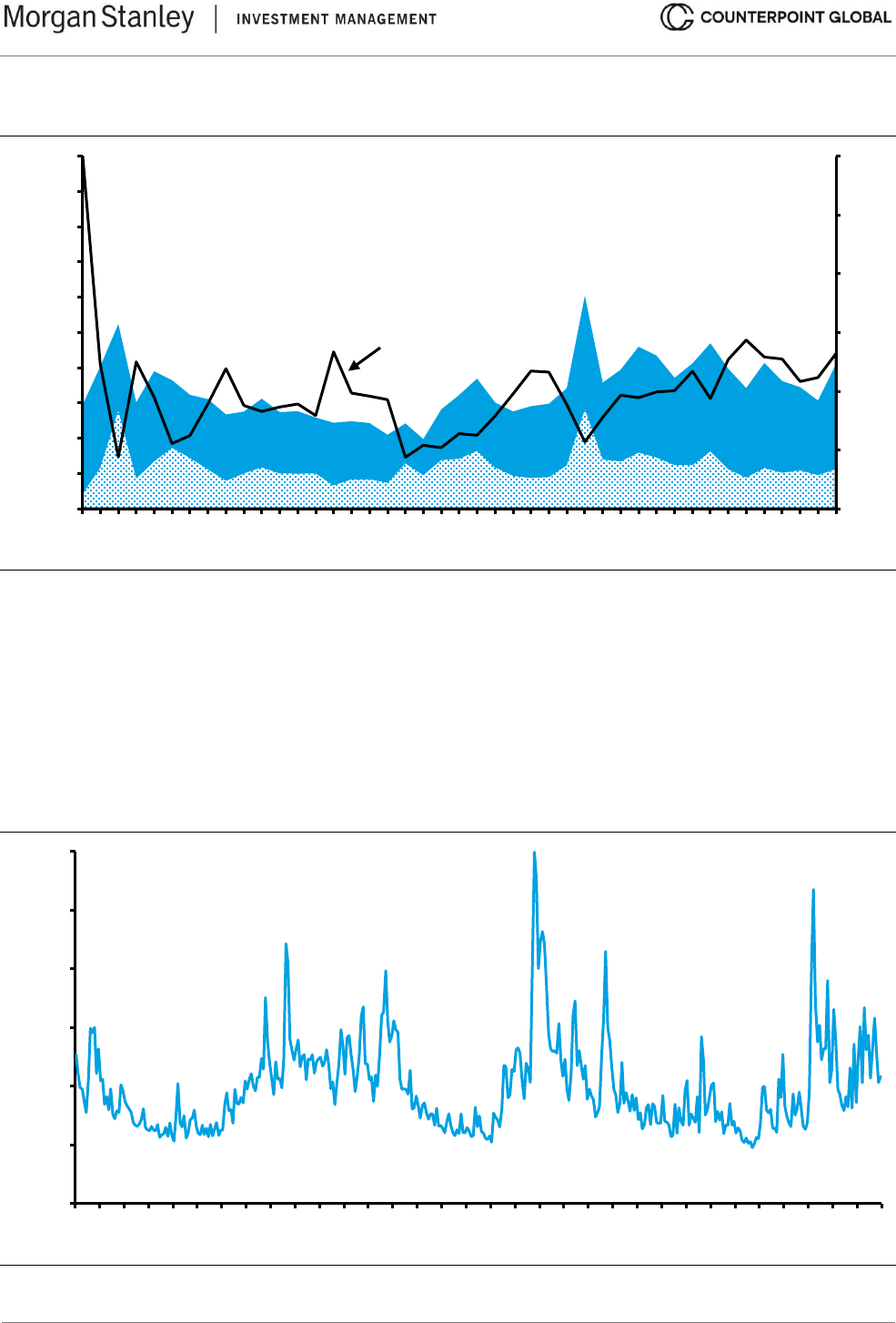
The Cboe Volatility Index (VIX) is a measure of the implied annual volatility of options on the S&P 500 Index and
is considered a gauge of collective risk aversion (see exhibit 11).
39
Generally, a rising VIX indicates an increase
in fear among investors and is consistent with poor stock market returns, and a decline in the VIX suggests a
decrease in fear and goes with good market results. Note the spikes in March 2009 as a result of the financial
crisis and in 2020 because of COVID.
Exhibit 11: Cboe Volatility Index (VIX), Monthly, 1990-2022
Source: FRED at the Federal Reserve Bank of St. Louis and Counterpoint Global.
Note: Data reflect end of month.
0
1
2
3
4
5
6
0%
2%
4%
6%
8%
10%
12%
14%
16%
18%
20%
1980
1981
1982
1983
1984
1985
1986
1987
1988
1989
1990
1991
1992
1993
1994
1995
1996
1997
1998
1999
2000
2001
2002
2003
2004
2005
2006
2007
2008
2009
2010
2011
2012
2013
2014
2015
2016
2017
2018
2019
2020
2021
2022
Equity Risk Premium / Baa Spread
Equity Risk Premium and Baa Spread
ERP /
Baa Spread
Equity Risk
Premium
Baa Spread
0
10
20
30
40
50
60
1990
1991
1992
1993
1994
1995
1996
1997
1998
1999
2000
2001
2002
2003
2004
2005
2006
2007
2008
2009
2010
2011
2012
2013
2014
2015
2016
2017
2018
2019
2020
2021
2022
Price

© 2024 Morgan Stanley. All rights reserved.
6422586 Exp. 2/28/2025
20
Credit spreads and the level of the VIX provide a proxy for collective risk aversion independent of the ERP. Low
spreads and volatility imply that investors are seeking risk, and high readings indicate fear of risky assets.
Low risk aversion translates into higher asset prices, holding constant the prospects for future cash flow. High
asset prices are associated with less upside and more downside in equity returns. Asset prices are often
vulnerable to decline when risk is perceived to be low. Examples include the spring of 2000, summer of 2007,
and fall of 2021. Asset prices are often very attractive when risk appears to be high, as we saw in March 2009
and March 2020.
The market places a price on other measures of risk that can be informative when considering the ERP. The
signals are strongest when the ERP, credit spreads, and VIX all indicate similar levels of extreme fear or greed.
Beta. Despite the CAPM’s popularity among practitioners, the concept of beta has been challenged on empirical
and intellectual grounds. The empirical problem is that beta does not predict expected returns the way it is meant
to. Specifically, stocks with low betas generate higher returns, and stocks with high betas deliver lower returns,
than the model predicts. The intellectual objection is that volatility in general, and beta in particular, are poor
ways to measure risk. Value investors generally define risk as potential permanent loss of capital and argue that
the volatility of asset prices does a poor job of capturing that risk.
We discuss methods to improve the measurement of beta and also review alternative approaches to estimating
the cost of equity. The objective is to come up with an estimate that captures the opportunity cost of equity
investors in a portfolio setting and that makes business, economic, and common sense.
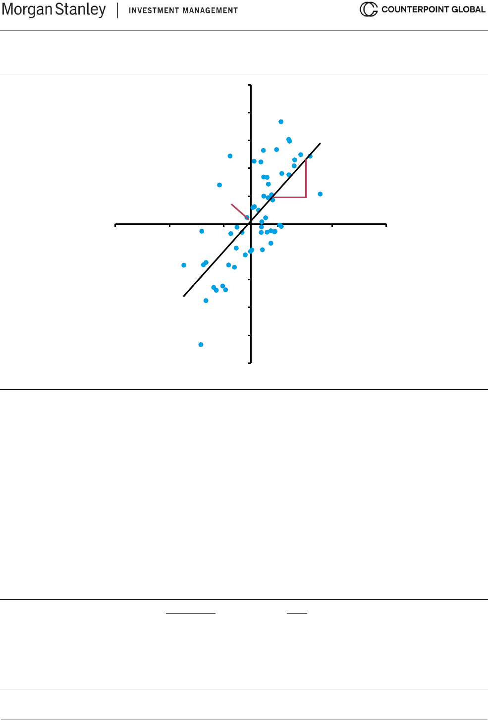
Beta measures the return of an individual security relative to the return on the market index. It reflects financial
elasticity. You calculate a historical beta by doing a regression analysis with the market’s total returns as the
independent variable (x-axis) and the asset’s total returns as the dependent variable (y-axis). The slope of the
best-fit line is the beta.
40
The slope of the regression line is the rise (up or down) over the run (left to right). The beta is 1.0 for a security
that goes up and down the same as the market. The beta is 2.0 for an asset that goes up or down at a percentage
twice that of the market. That asset is considered to be riskier than the market. The beta is 0.5 if the security
rises and falls at a rate that is one-half of the market’s percentage. That security is less risky than the market.
Exhibit 12 shows the beta for Nike, a sportswear company, using monthly returns over the 60 months ended
2022, and the S&P 500 as the index. The beta is 1.09. The equation for the “slope intercept form” of a straight
line is y = mx + b. In this equation, which appears in the top right corner of exhibit 12, “m” equals beta (slope)
and “b” is alpha (intercept). Alpha is the y-intercept of a regression line and as such captures the excess return.
If you combine all of the assets in an index and correlate it versus the index itself, you will get a beta of 1.0 and
an alpha of zero before consideration of any costs.
© 2024 Morgan Stanley. All rights reserved.
6422586 Exp. 2/28/2025
21
Exhibit 12: Beta and Alpha for the Stock of Nike, 60 Months Through 2022
Source: FactSet.
Similar to the ERP, beta should be a measure that looks forward but is unobservable. As a result, to estimate it
we have to examine historical relationships and make adjustments to remove some of the noise.
Calculating beta requires a number of judgments. These include which index to compare to, how far back in
history to go, and whether to measure frequency on a daily, weekly, monthly, quarterly, or yearly basis.
The benchmark the marginal buyer of the security is likely to use is a good way to think about the appropriate
index for comparison. The S&P 500 is a sensible candidate for investors in the United States as it is by far the
most common benchmark. The beta will vary based on the benchmark. Exhibit 13 shows the beta for Nike (60-
month, using monthly returns) calculated for four indexes. The betas are clustered for the indexes based in the
U.S., but the figure increases to 1.25 using the MSCI ACWI, a global equity index captures the performance of
nearly 3,000 large- and mid-capitalization stocks in 23 developed and 24 emerging markets.
Exhibit 13: Nike’s Beta Using Four Benchmarks
Relative to: Beta
S&P 500 1.09
Russell 1000 1.07
Dow Jones 1.07
MSCI ACWI 1.25
Source: FactSet and Counterpoint Global.
Note: Monthly returns over the 60 months ended 2022.
y = 1.09x + 0.50
-25
-20
-15
-10
-5
0
5
10
15
20
25
-25 -15 -5 5 15 25
Nike Monthly Returns (Percent)
S&P 500 Monthly Returns (Percent)
Intercept = Alpha
Slope = Beta

© 2024 Morgan Stanley. All rights reserved.
6422586 Exp. 2/28/2025
22
Another decision is how far back to go in time. The benefit of going back further is that there are more data and
the regression result is more reliable as a result. The drawback is that the company may have changed its
business model, business mix, or levels of financial leverage. Or it may have simply matured. Longer is better
for companies with stable business models and capital structures. Calculate a rolling beta if you sense that data
from the past fail to reflect the present. You can consider a shorter period if the beta changes materially during
the period you measure.
Exhibit 14 shows the betas for Nike using the S&P 500 and monthly returns over four different time horizons.
Here again, the figures for three to seven years are close to one another. There is a modest drop only at 10
years. The exhibit also shows the strength of the correlation, R-squared, between the returns for the market and
the stock in each period. The correlations weaken the further you look back.
Exhibit 14: Nike’s Beta Using Four Time Periods
Measurement period Beta R-squared
Three years 1.10 49%
Five years 1.09 49%
Seven years 1.06 43%
Ten years 1.00 37%
Source: FactSet and Counterpoint Global.
Note: Monthly returns over the 60 months ended 2022.
The frequency of the measurement is the last choice. More frequent measurement creates more data. However,
McKinsey’s book on valuation and work by Aswath Damodaran both suggest biases associated with daily or
weekly data for beta estimation.
41
McKinsey recommends monthly data, and Damodaran recommends using
high-frequency data only with certain adjustments. A good place to start is monthly returns over 60 months.
Exhibit 15 shows Nike’s beta relative to the S&P 500 using daily, weekly, monthly, quarterly, and yearly
frequencies over five years. The results are in the range of 1.03 to 1.09 except for the quarterly measure. Also
included are the standard errors.
Exhibit 15: Nike’s Beta Relative to the S&P 500 Using Five Measurement Frequencies
Frequency Beta Standard error
Daily 1.07 0.03
Weekly 1.09 0.07
Monthly 1.09 0.15
Quarterly 1.28 0.26
Yearly 1.03 0.45
Source: FactSet and Counterpoint Global.
Note: Returns over the 5 years ended 2022.
The process is imprecise even with thoughtful choices in calculating the historical beta. For instance, Amazon’s
60-month raw beta versus the S&P 500 based on monthly returns is 1.22 with an R
2
of 44 percent and a standard
error of 0.18. These figures suggest you can be 95 percent confident that Amazon’s beta is somewhere between
0.86 and 1.58, which reveals the imprecision of a single number. There are a few ways to improve the estimate
of beta.

© 2024 Morgan Stanley. All rights reserved.
6422586 Exp. 2/28/2025
23
Adjusted Beta. The first method regresses the beta toward 1.0 to create an adjusted beta. Bloomberg and
Value Line use this technique. Here’s the formula that is commonly used:
Adjusted beta = Raw beta (0.67) + 1.0 (0.33)
So, for example, Amazon’s adjusted beta is 1.15 ([1.22*.67]) + [1.0*.33]).
The justification for this adjustment is the empirical evidence that betas tend toward 1.0 over time.
42
This makes
economic and intuitive sense. The value of a company can be broken down into a steady-state value and the
present value of growth opportunities (PVGO).
43
The steady-state value comes from assets in place and reflects
the cash flows the business currently generates. The PVGO reflects the expected value of future investments
that create value.
The value of most companies is a combination of the two, and as a company matures the steady-state
contributes more to value and the PVGO adds less. Research shows that the investments in the PVGO are
riskier than the assets in place. That means they have higher betas. As the mix of firm value shifts from PVGO
toward steady-state, the beta drifts lower.
44
This adjustment is reasonable but applying proper weights is a challenge. The rate at which betas converge to
1.0 is different from one company to the next. But overall, some regression in the beta toward 1.0 generally
improves the estimate of a beta that seeks to reflect future risk.
Acknowledging that betas regress is especially important in calculating a continuing value. In a DCF model, the
continuing value is an estimate of the value beyond the explicit forecast period. Healthy businesses tend to
become larger, more profitable, and more stable as they mature. That means that the cost of capital used to
estimate the continuing value should reflect the business characteristics in the future versus what they are today.
Industry Beta. Another way to improve beta is to use an industry beta rather than the beta of an individual
company. The economic rationale is that business risk, or variability of cash flows, will be similar for all
companies within an industry. An industry beta can reduce error by using a larger sample, potentially cancelling
the noise that appears in the estimation of beta for individual companies.
The calculation of an industry beta has three steps:
1. Unlever the beta. A company’s beta combines business risk and financial risk. We want to measure business
risk first, so we need to remove the effect of financial leverage from the beta. The equation to unlever the beta
is based on M&M’s invariance proposition:
45
β
U
= β
L
/[1 + (1 – T) D/E)]
Where:
β
U
= Beta unlevered
β
L
= Beta levered
T = Tax rate
D = Market value of debt
E = Market value of equity

© 2024 Morgan Stanley. All rights reserved.
6422586 Exp. 2/28/2025
24
To illustrate, consider the stock of a company with a raw beta of 1.2, a 25 percent tax rate, and 20 percent debt
and 80 percent equity (note that D/E is not the ratio of debt to total capital but of debt to equity):
β
U
= 1.2/[1 + (1 – .25) .20/.80)]
= 1.2/[1 + .75(.25)]
= 1.2/1.1875
β
U
= 1.0
2. Calculate the average beta for the industry. The trick here is defining the industry. Ideally, it is a group of
companies with similar business risk because they are exposed to the same markets, create comparable
products, and deal with similar customers. The average can be weighted by market capitalization, and
calculating the median helps check for potential outliers that might distort the average.
3. Relever the beta for the specific company. Unlevering the beta isolates business risk, which is considered
uniform for companies within the same industry. We must now reintroduce financial risk, which can vary for
companies within the same industry. Financial risk is estimated using a company’s expected long-term capital
structure. The formula to relever the beta is:
β
L
= β
U
[1 + (1 – T) D/E]
Take for example a company that has an industry beta of 1.05, a 20 percent tax rate, and 25 percent debt and
75 percent equity:
β
L
= 1.05 [1 + (1 – .20) .25/.75)]
= 1.05 [1 + .80(.333)]
= 1.05 [1.267]
β
U
= 1.33
The motivation to calculate an industry beta is to come up with a more accurate and stable estimate of a
company’s risk. But there is not a great deal of evidence that industry betas are much better than firm-specific
betas as they face a lot of the same analytical issues.
46
Further, many companies operate in multiple lines of
business and estimating the risk for each is cumbersome, even if it provides an improved estimate of beta.
47
Aswath Damodaran provides his estimates of levered and unlevered betas for dozens of industries and includes
a correction for industries with lots of cash. When cash exceeds debt, a company has negative financial risk.
This dampens the volatility of cash flows and lowers the risk for shareholders.
Winsorized Beta. Ivo Welch, a professor of finance, finds the predictive value of beta improves when past
returns are winsorized.
48
Winsorizing removes extreme values in a data series to reduce the impact of non-
representative outliers.
Using daily returns, data are cut off at -2 times and +4 times the market’s return. For instance, if the market’s
return on one day is +5 percent, the stock’s returns are winsorized at -10 and +20 percent. If the market is down
5 percent, the returns are winsorized at -20 to +10 percent. This process changes the slope of the regression
and hence the beta.
Welch finds that this modification produces a beta that better predicts future betas than does a simple regression
or a regression combined with an adjustment.

© 2024 Morgan Stanley. All rights reserved.
6422586 Exp. 2/28/2025
25
The cost of equity is an opportunity cost that is implicit and therefore difficult to pin down with precision. But all
is not lost. There are procedures, including comparing figures to other measures that are set by the market and
applying business sense, that can allow for a useful calculation. Remember, too, that what determines a great
investment is how the expectations for future cash flows change over time. The biggest driver of expectations is
business results.
To summarize this section, we recommend using the 10-year Treasury note as the risk-free rate, an equity risk
premium that looks forward, and a 60-month, monthly beta that is adjusted as appropriate. Each calculation is
open to debate but this is a good starting point. Estimates for the cost of equity should also be checked by
examining other forms of risk priced by the market.
© 2024 Morgan Stanley. All rights reserved.
6422586 Exp. 2/28/2025
26
Weighted Average Cost of Capital
The weighted average cost of capital (WACC) combines the opportunity cost of the sources of capital with the
relative contribution of those sources based on target weights.
We can start with the simple example of a company funded solely with debt and equity. Assume an after-tax
cost of debt of 5 percent and a cost of equity of 10 percent that is financed with 20 percent debt and 80 percent
equity. The weighted average cost of capital would be 9.0 percent, calculated as follows:
WACC = (cost of debt × weighting of debt) + (cost of equity × weighting of equity)
= (5% × 20%) + (10% × 80%)
= 1.0% + 8.0%
= 9.0%
Exhibit 16 shows an estimate of WACC for companies in the Russell 3000, a good proxy for the overall U.S.
equity market, from 1985 to 2022. We use Aswath Damodaran’s estimates for the cost of equity, the yield on
Baa-rated bonds as a proxy for the pre-tax cost of debt, the overall effective corporate tax rate, and the aggregate
debt-to-total capital ratio from each year. The average WACC over the full period was 7.9 percent, and the
estimate at the end of 2022 was 8.8 percent.
Exhibit 16: Weighted Average Cost of Capital for the Russell 3000, 1985-2022
Source: FactSet; Moody’s; Aswath Damodaran; FRED at the Federal Reserve Bank of St. Louis; Counterpoint Global
estimates.
Note: Excludes financials and real estate; Capital structure reflects book value of total long- and short-term debt and market
value of equity; cost of debt is the Moody's Seasoned Baa Corporate Bond Yield; cost of equity = yield on 10-year U.S.
Treasury note + equity risk premium.
The weighted average cost of capital is the appropriate rate at which to discount the future free cash flows
attributable to the firm to determine their present value. This is called free cash flow to the firm (FCFF).
When discounting cash flows attributable to equity holders, which is common practice for financial services firms,
the correct discount rate is the cost of equity capital. This is called free cash flow to equity (FCFE). Practitioners
report that they use the FCFF model roughly twice as frequently as the FCFE model.
49
0
2
4
6
8
10
12
1985
1986
1987
1988
1989
1990
1991
1992
1993
1994
1995
1996
1997
1998
1999
2000
2001
2002
2003
2004
2005
2006
2007
2008
2009
2010
2011
2012
2013
2014
2015
2016
2017
2018
2019
2020
2021
2022
Percent
Average
© 2024 Morgan Stanley. All rights reserved.
6422586 Exp. 2/28/2025
27
There are a number of items to bear in mind when estimating the WACC:
• Weighting of debt and equity should be based on market values and not book values. The reason is that
opportunity cost is based on the prevailing asset price rather than the level at which the company reflects
debt or equity on the balance sheet. Indeed, some companies have negative equity as the result of the
vagary of accounting.
50
Companies sometimes share a target for the debt-to-total capital ratio based on book values. In those
instances, you should translate the target into one based on market values. Most companies try to stay
close to their target capital structures. But use the target weights of debt and equity even if the current
weights are different because you want the best estimate of what the capital structure will look like over
time.
Exhibit 17 shows the debt-to-total capital ratio for the Russell 3000 from 1985 to 2022. The 2022 figure
was 18 percent, below the 30 percent average over the full period. The decline in leverage levels since
2008 notwithstanding, the trend in the U.S. over the last century has been to increase leverage.
51
There
is also evidence that companies adjust their capital structures in reaction to changes in tax rates.
52
Exhibit 17: Debt-to-Total Capital Ratio for the Russell 3000, 1985-2022
Source: FactSet and Counterpoint Global estimates.
Note: Excludes financials and real estate; Capital structure reflects the book value of total long- and short-term debt and the
market value of equity.
• The WACC is the discount rate a company should use for investments that have risk consistent with the
underlying business. Companies and investors sometimes evaluate the attractiveness of an investment
using the cost of funding rather than the cost of capital, especially in cases where the investment is
expected to add to earnings per share. This is incorrect.
However, the discount rate for an investment that is more or less risky than that of the company should
be higher or lower than the company’s overall WACC to reflect that difference. Empirically, companies
commonly stick to one cost of capital, which introduces the risk of overinvesting in high-risk investments
and underinvesting in low-risk investments.
53
0
5
10
15
20
25
30
35
40
45
50
1985
1986
1987
1988
1989
1990
1991
1992
1993
1994
1995
1996
1997
1998
1999
2000
2001
2002
2003
2004
2005
2006
2007
2008
2009
2010
2011
2012
2013
2014
2015
2016
2017
2018
2019
2020
2021
2022
Percent
Average

© 2024 Morgan Stanley. All rights reserved.
6422586 Exp. 2/28/2025
28
• Don’t adjust your WACC to do scenario analysis. The discount rate should be consistent. You reflect
the range of values by considering different potential outcomes for cash flows.
The expectations infrastructure is an analytical tool that can help create scenarios. It starts with “value
triggers,” including sales growth, operating costs, and investments, and considers how changes in those
triggers ultimately affect sales, operating profit margin, and investment rate. The key is the value triggers
are refined by considering “value factors,” six microeconomic determinants of the ultimate value drivers.
The expectations infrastructure guides analysis of how potential changes in value triggers flow through
value factors in order to determine value.
54
A careful examination of the probabilities and values of the various scenarios is the way to capture and
assess risk. Financial executives are notoriously poor forecasters and incorrectly compensate for that
deficiency by using a hurdle rate that tacks on a premium of about six percentage points to the cost of
capital.
55
• The WACC should be updated relatively frequently. Companies and investors should have a current
sense of opportunity cost and what that means for the opportunity set of investment possibilities.
Companies tend to be slow to change their cost of capital estimates, often reviewing the calculation
annually.
56
A lot can change in a year.
• The adjusted present value (APV) method is useful if you expect a company’s capital structure to change
over time. For example, this approach is relevant for a company that levers up and expects to pay down
debt rapidly. (See appendix A for a discussion of the approach.) APV relies on the principle of additivity.
You value a company as if it were financed solely with equity, value the tax shield, and then add the
parts to determine corporate value.
The WACC may include other forms of financing, including convertible bonds and preferred equity. But these
are small relative to straight debt and equity.

© 2024 Morgan Stanley. All rights reserved.
6422586 Exp. 2/28/2025
29
Other Forms of Financing
Debt and equity are by far the largest sources of capital for U.S. public companies. As of the end of 2022, the
total value of corporate debt and leases was about $10 trillion and the market value of equity was approximately
$40 trillion. Companies use other forms of external financing as well, such as convertible debt and preferred
stock. The size of the convertible debt market was $240 billion based on market value, and $250 billion based
on par value, in 2022. The value of preferred stocks in 2022 was roughly $310 billion for stocks listed on major
exchanges, and $540 billion including stocks that trade over-the-counter (OTC). Federal National Mortgage
Association and Federal Home Loan Mortgage Corporation, known as Fannie Mae and Freddie Mac, account
for nearly all of the OTC issuance.
Convertible Bonds. Convertible bonds combine a straight debt issue with a warrant. A warrant provides the
owner with the right, but not the obligation, to buy the stock at a specified exercise price by a certain date.
Warrants, unlike options, are for the issuance of new shares. That means that current shareholders are diluted
if the convertible holders exercise the warrants. In the calculation of a company’s capital structure, the bond
portion is debt and the warrant is equity.
Convertible bonds generally have a lower yield than straight debt because the attached warrant has value. Many
issuers of convertible bonds have relatively high equity volatility. This makes sense because volatility is a large
driver of warrant value. It is common for convertible bonds to be junior to other debt in the capital structure.
The market value of convertible bonds falls into one of three broad regimes. The first is when the stock price is
well above the exercise price. Here, convertible bonds trade more like straight equity than debt. Second, when
the stock price is close to the exercise price the bond value and warrant are both meaningful sources of value.
Finally, when the stock price falls well below the exercise price the convertible bond is “busted,” and trades at a
yield similar to straight debt.
When the stock price is close to the strike price it is vital to value the debt and warrant properly. To value the
straight bond, you proceed as if warrant does not exist. You apply the rate of interest the company would need
to pay if it had issued a straight bond. The warrant can be valued using a standard warrant pricing model. The
implied volatility of the stock is a key input. Then you add the debt and warrant values to estimate the value of
the convertible bond.
Preferred Stock. Preferred stock is an equity instrument that combines the features of debt and equity. Similar
to debt, preferred stock typically provides its holder a stream of cash flows in the form of a dividend. Preferred
stock, similar to debt, generally has no voting rights. Like equity, the company has no contractual obligation to
pay a dividend on preferred stock and the board of directors has discretion in setting the preferred dividend. But
companies have to pay the specified dividends on preferred stock before they pay dividends on common stock.
Preferred stock is junior to debt but senior to common equity in the capital structure. As a result, the cost of
preferred stock is typically somewhere in between the two. Preferred stock also has a senior claim to common
equity in liquidation. The cost of preferred stock equals the preferred dividend per share divided by the market
price per share. For example, cost of preferred stock is 8.75 percent for an issue paying a dividend of $1.75 per
year and a price of $20 (8.75 = $1.75 ÷ $20).
Unlike most interest payments on debt, dividends on preferred stock are not tax deductible for the issuing firm.
This deters a lot of companies from issuing preferred stock. The largest issuers are financial institutions, real
estate investment trusts (REITs), and public utilities.

© 2024 Morgan Stanley. All rights reserved.
6422586 Exp. 2/28/2025
30
It is attractive for companies to own the preferred stock of other companies because the tax laws allow corporate
owners to exclude 70 percent of dividend income from their taxable income. This is especially valuable because
the yields on preferred stock tend to be higher than the yields on common stock. Financial companies sometimes
use preferred stock to improve capital ratios at a cost lower than straight equity.
Most preferred issues include some provision for retirement. For example, preferreds frequently offer an option
to retire the issue, convert it into common stock, or repurchase it at a specific time and price. This means that
some preferred issues have an embedded option that should be included in valuation.

© 2024 Morgan Stanley. All rights reserved.
6422586 Exp. 2/28/2025
31
Optimal Capital Structure
A company’s optimal capital structure finds the trade-off between the financial benefits of debt and the risk of
financial distress that maximizes the value of the firm.
Corporate tax policies in many countries favor debt over equity financing. Specifically, equity is subject to
taxation at the corporate and individual levels. Individuals must pay taxes on dividends and capital gains in taxable
accounts. In fact, share buybacks, another means to return cash to shareholders, are subject to triple taxation
in the U.S. following the Inflation Reduction Act of 2022, which introduced a one percent excise tax on buybacks.
Most countries treat some percentage of interest expense as a cost of doing business that a company may
deduct from income before paying taxes. This avoids the problem of double taxation. As a result, debt financing
is sensible for many companies because it increases the value of the firm by making additional cash flow
available for the providers of capital.
Some debt may add value but it stands to reason that too much debt introduces the risk of financial distress.
The question is how companies actually behave relative to what might be assessed as ideal.
Surveys of financial executives reveal some interesting evidence. First, companies generally adopt a target
capital structure with debt less than the optimal amount because they want to ensure sufficient resilience.
Further, a relatively recent survey found that only 24 percent of the chief financial officers of large corporations
cited interest deductibility as an important factor in determining debt levels.
This result, which is down from 60 percent in a comparable survey from 2001, suggests that that the value of
the tax shield is not the guiding factor in setting a target capital structure. That said, federal tax rates and interest
rates are lower today than they were at the beginning of this century.
57
There are a couple of popular approaches to studying capital structure.
Trade-Off Theory. This theory says the optimal capital structure is the ideal trade-off between the benefit of
interest tax shields and the cost of financial distress (see exhibit 18). When there is no debt, you can value the
firm using an estimate of the cost of equity and an unlevered beta. As a company adds debt (moving to the right
on the x-axis), the benefit of the tax shield initially rises at a rate faster than the cost of financial distress.
Exhibit 18: Trade-Off Theory of Optimal Capital Structure
Source: Based on Stewart C. Myers, “The Capital Structure Puzzle,” Journal of Finance, Vol. 39, No. 3, July 1984, 575-592.
Interest tax
shield minus
cost of financial
distress
Market
Value of
Firm
Optimum
Debt
Value with all-equity financing
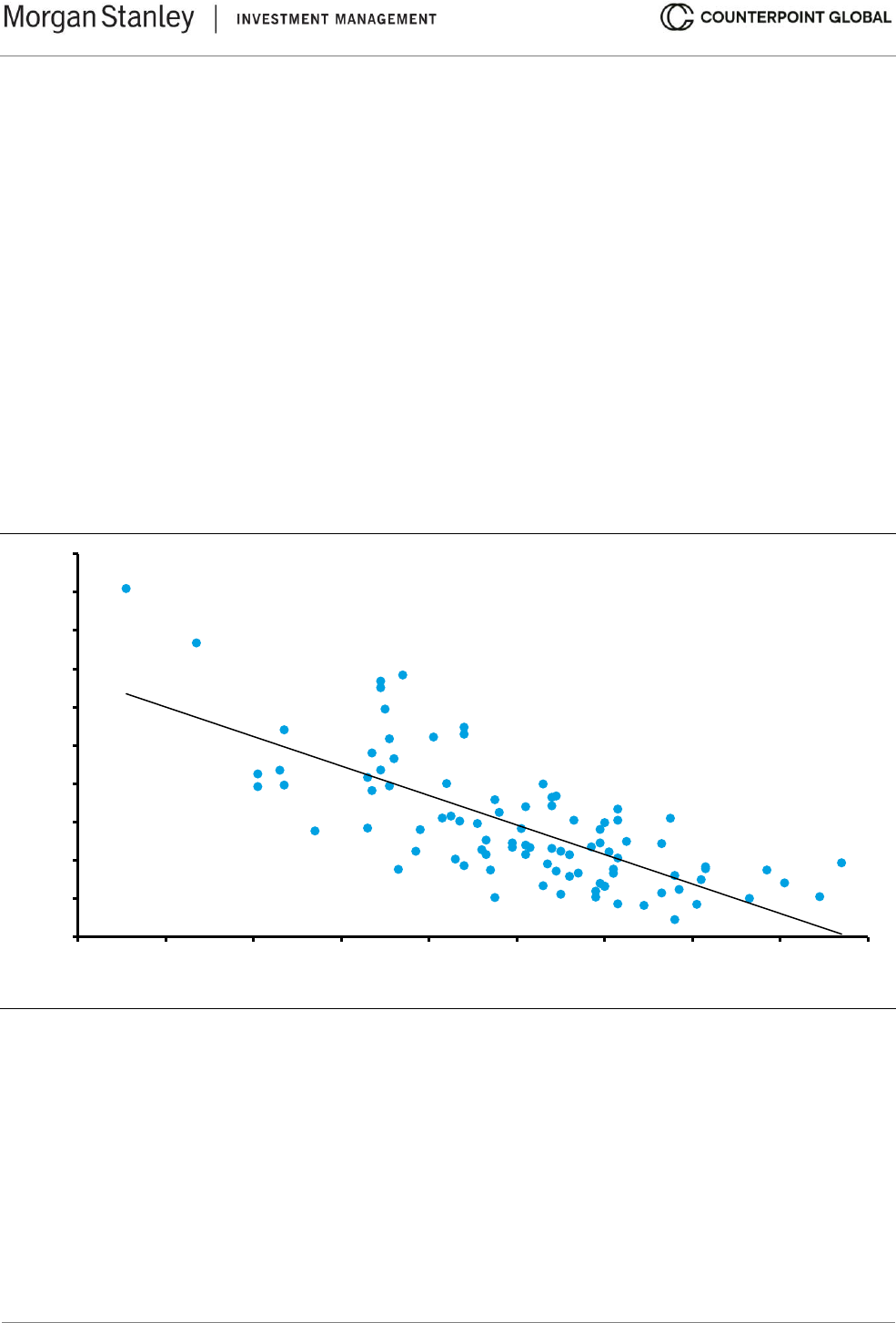
© 2024 Morgan Stanley. All rights reserved.
6422586 Exp. 2/28/2025
32
But at some point, the cost of financial distress exceeds the benefit of the tax shield and incremental debt
reduces firm value. One way to think about it is that interest expense becomes a fixed cost, and therefore
declines in operating profit create pre-tax losses. A company must pay taxes for the tax shield to be of value.
Adding debt therefore increases the probability that a company will be unprofitable and unable to benefit from
tax shields.
We already saw that many companies have a target capital structure that is more conservative than what the
trade-off theory would advise. Yet some high level data advise the concept is useful.
For example, the theory proposes that businesses with low business risk are good candidates to use debt.
Business risk reflects the volatility of operating profits and is measured with unlevered beta. The use of debt can
be quantified with the ratio of debt to total capital. Aswath Damodaran provides these data. Exhibit 19 shows the
relationship between unlevered beta and the ratio of debt to total capital for more than 90 industries using
Damodaran’s figures. As the theory predicts, companies with low business risk tend to have higher debt-to-total
capital ratios than businesses with high business risk.
Exhibit 19: Unlevered Beta and Debt-to-Total Capital Ratios by Industry
Source: Aswath Damodaran and Counterpoint Global.
The trade-off theory also helps explain the rise of the leveraged buyout industry in recent decades. A leveraged
buyout is a transaction where a financial sponsor buys a company that has solid and stable cash flows and
finances the deal with a high ratio of debt to equity. The framework also explains why companies raise equity
when financial distress increases and why companies beyond the optimal debt-to-total capital ratio can add
value by paying down debt.
58
But the theory fails to explain other facts, including why capital structures vary substantially within industries and
why companies are not proactive in changing their policies to reflect the drivers of the theory, including changes
in the cost associated with financial distress as well as changes in interest and tax rates.
0
10
20
30
40
50
60
70
80
90
100
0.0 0.2 0.4 0.6 0.8 1.0 1.2 1.4 1.6 1.8
Debt-to-Total Capital (Percent)
Unlevered Beta
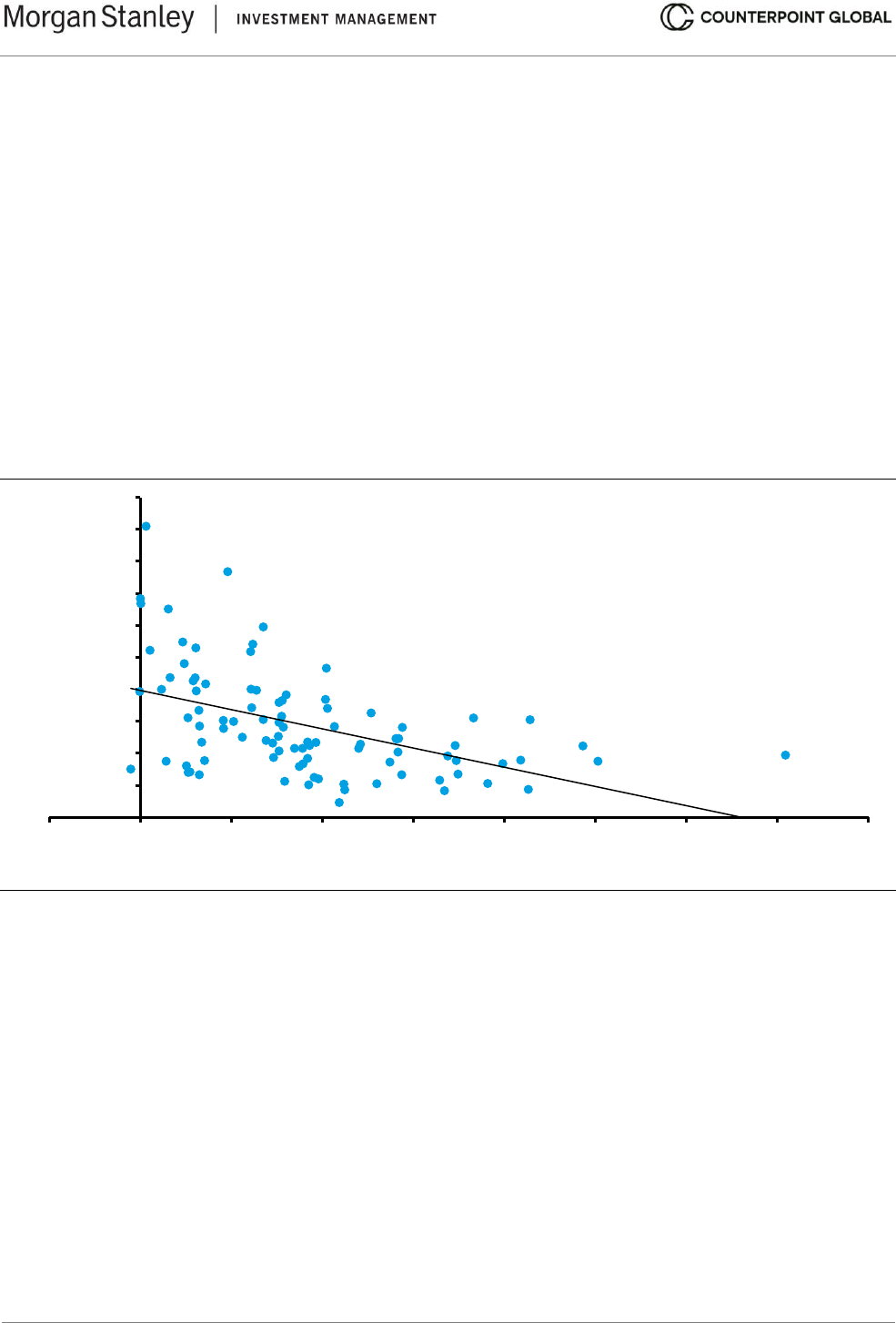
© 2024 Morgan Stanley. All rights reserved.
6422586 Exp. 2/28/2025
33
Pecking Order Theory. Companies finance their operations internally through cash from operations or externally
by raising debt or equity. This theory assumes that companies prefer internal finance, but if those funds are
insufficient firms will raise capital following a pecking order from the least to most risky capital.
59
Specifically,
they will start with internal financing, followed by debt, and finally with equity. Capital structure decisions are not
motivated by the value of the tax shields but are related to the economics of the business.
A company can rely on internal financing when its growth rate is equal to or lower than its return on invested
capital (ROIC). This allows us to test the pecking order theory because, holding growth constant, we should see
businesses with high ROICs have lower debt-to-total capital ratios than businesses with low ROICs.
Exhibit 20 again uses Damodaran’s data to examine this relationship for more than 90 industries. While far from
perfect, the basic pattern holds true. Indeed, many of the best businesses in the world, as measured by ROIC,
have very conservative capital structures.
Exhibit 20: Industry ROIC and Debt-to-Total Capital Ratio
Source: Aswath Damodaran and Counterpoint Global.
These theories particularly apply to companies that have capital structures that are expected to remain roughly
static. Valuing dynamic capital structures requires a tool such as adjusted present value (see appendix A).
Here are some final thoughts that are more speculative. One way to think about the impact of taxes on the cost
of capital is to consider the government as a stakeholder. Use of debt lowers the value of the government’s claim
on cash flows and increases the value to debt and equity holders.
In the U.S., corporate taxes as a percentage of total federal revenue have drifted lower from a peak of nearly 40
percent in 1943 to 9 percent today (see exhibit 21). There are several factors that explain this drop. The first is
that corporate leverage was near its historic low in the 1940s and has risen steadily in the last century or so.
0
10
20
30
40
50
60
70
80
90
100
-10 0 10 20 30 40 50 60 70 80
Debt-to-Total Capital (Percent)
Return on Invested Capital
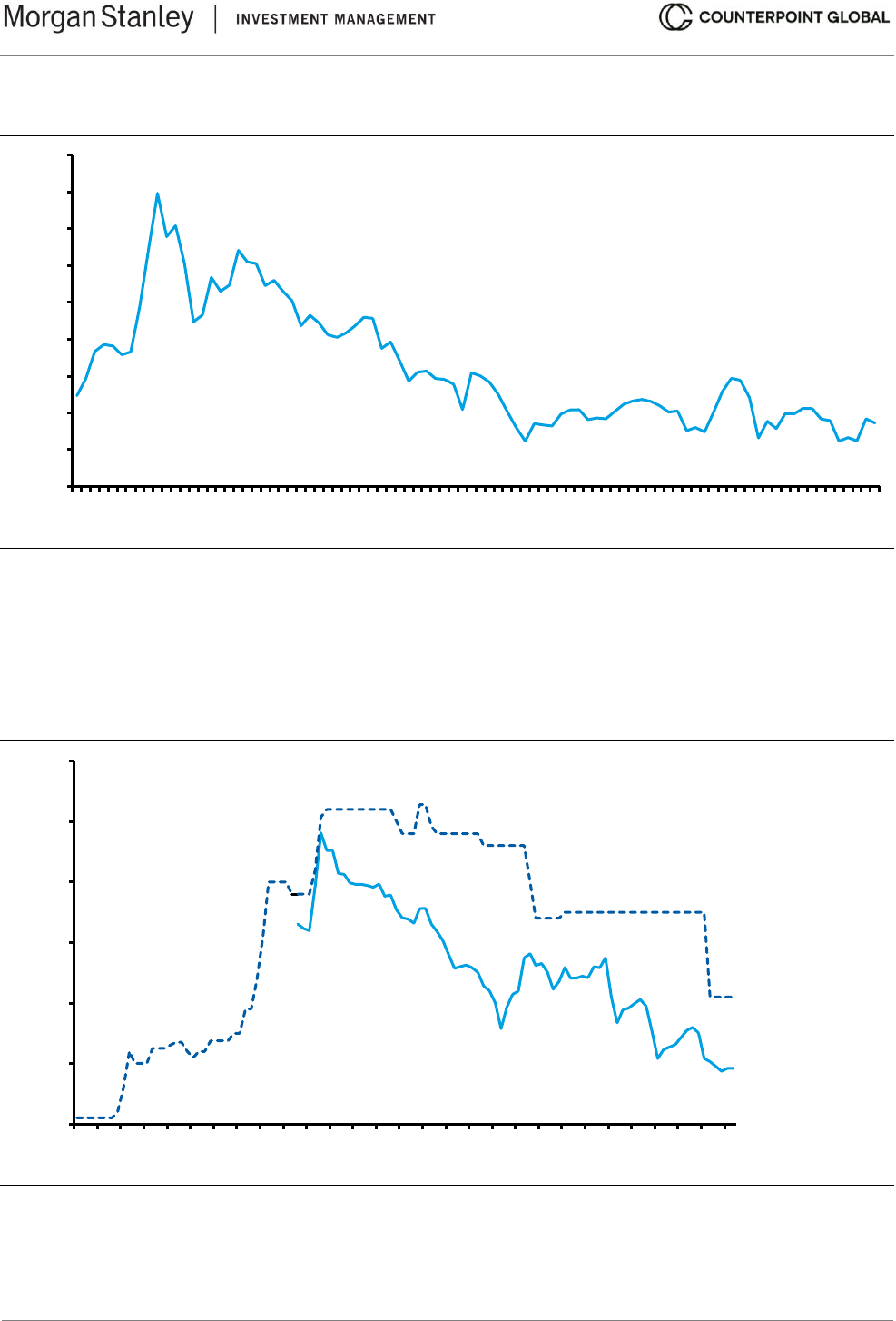
© 2024 Morgan Stanley. All rights reserved.
6422586 Exp. 2/28/2025
34
Exhibit 21: Corporate Taxes as Percentage of Federal Tax Revenue, 1934-2022
Source: www.govinfo.gov/ and Counterpoint Global.
Second is that the top marginal and effective tax rates were higher in the past than they are today. Exhibit 22
tracks the top federal statutory tax rate for U.S. corporations from 1909 to the present, and the effective tax rate
since 1947. The top marginal rate exceeded 50 percent for stretches during the 1950s and 1960s but has
descended to today’s 21 percent rate, which went into effect in 2018.
Exhibit 22: Top Federal Statutory and Effective Tax Rates for U.S. Corporations, 1909-2022
Source: Tax Policy Center; FRED at the Federal Reserve Bank of St. Louis; Counterpoint Global.
Another reality is the operations of large American companies have become more global over time. That
provides them with the opportunity to manage where their profits are taxed, hence lowering the overall tax rate
they pay.
0
5
10
15
20
25
30
35
40
45
1934
1936
1938
1940
1942
1944
1946
1948
1950
1952
1954
1956
1958
1960
1962
1964
1966
1968
1970
1972
1974
1976
1977
1979
1981
1983
1985
1987
1989
1991
1993
1995
1997
1999
2001
2003
2005
2007
2009
2011
2013
2015
2017
2019
2021
Percent
0
10
20
30
40
50
60
1909
1913
1917
1921
1925
1929
1933
1937
1941
1945
1949
1953
1957
1961
1965
1969
1973
1977
1981
1985
1989
1993
1997
2001
2005
2009
2013
2017
2021
Percent
Effective tax rate
Top federal
statutory tax rate
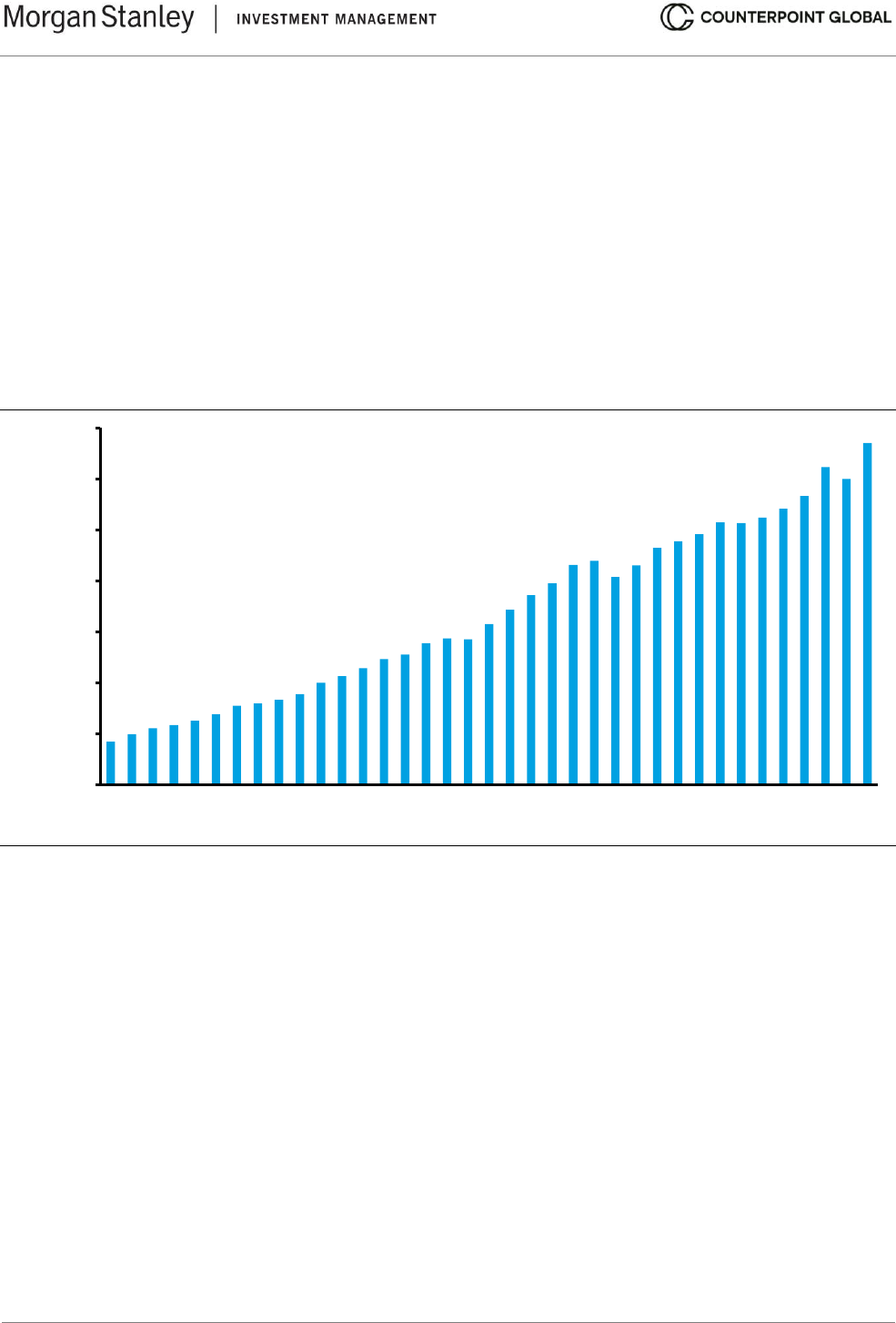
© 2024 Morgan Stanley. All rights reserved.
6422586 Exp. 2/28/2025
35
But perhaps the biggest and least discussed tax shield is the rise in intangible investment. The important
observation is that companies expense intangible investments on their income statement and therefore reduce
pre-tax profit. Companies capitalize tangible investments, which means they record them on the balance sheet
and depreciate them on the income statement over the asset’s estimated useful life. An intangible and tangible
investment of the same magnitude and payback can have very different tax treatment.
Exhibit 23 shows our estimate of the investment component of selling, general, and administrative costs (SG&A)
excluding research and development (R&D) for companies in the Russell 3000 excluding financial and real
estate firms. The total was more than $1.3 trillion in 2021.
60
An intangible investment is a discretionary outlay in
pursuit of growth that creates value. That expense lowered pre-tax income, taxes, and net income.
Exhibit 23: Investment SG&A ex-R&D for the Russell 3000, 1985-2021
Source: FactSet; Aneel Iqbal, Shivaram Rajgopal, Anup Srivastava, and Rong Zhao, “Value of Internally Generated
Intangible Capital,” Working Paper, February 2022; Counterpoint Global.
Note: Excludes financial and real estate companies.
We need to treat intangible and tangible investments the same way in order to compare them properly. In this
case, we capitalize investment SG&A ex-R&D and amortize it over an appropriate period. We estimate that
would have increased the pre-tax earnings for companies in the Russell 3000 by about $360 billion in 2021.
Applying a 21 percent tax rate would yield about $75 billion in additional corporate tax revenue, all else held
equal. Compare that to the $372 billion in federal taxes that companies paid in 2021.
0
200
400
600
800
1,000
1,200
1,400
1985
1987
1989
1991
1993
1995
1997
1999
2001
2003
2005
2007
2009
2011
2013
2015
2017
2019
2021
Amount ($ Billions)

© 2024 Morgan Stanley. All rights reserved.
6422586 Exp. 2/28/2025
36
Conclusion
The cost of capital is a measure of expected return that reflects compensation for deferring consumption. It
allows us to estimate values in the future via compounding and bring future values to the present via discounting.
You can think of it as a form of opportunity cost.
Pinpointing the cost of capital is a challenge because while most practitioners agree on the theoretical framework
there is wide discretion in how it is applied. As a result, the output can vary widely.
61
Combine this with the fact
that the inputs move around and it is easy to see why many investors throw up their hands in frustration.
Our view is a little more optimistic. The main idea to remember is that we are trying to estimate a discount rate
that is sound and that makes business and common sense. To that end, we can use risks that are priced by the
market to guide our judgment.
The cost of debt is relatively straightforward to calculate because the terms of borrowing are set by contract and
required yields are visible. This is particularly true for debt rated as investment grade. For debt rated below
investment grade the task is more challenging because of the risk of default and uncertainty of what creditors
may recover in that case.
The cost of equity is difficult to estimate because it has an implicit cost. In other words, investors expect a certain
rate of return even if it is not spelled out explicitly. The two main hurdles in estimating the cost of equity properly
are an estimate of the equity risk premium, the excess compensation over time for owning equities relative to a
risk-free asset, and the contribution of a firm’s risk to a portfolio.
We find the estimates for the ERP that Aswath Damodaran produces every month to be a sound starting point.
Further, Damodaran provides a spreadsheet that allows an investor to use his or her assumptions and to modify
them to taste. The relationship between his ERPs and subsequent returns for the market over 10 years are
reasonable.
How a stock affects the risk of a portfolio, which beta seeks to measure, is more difficult and controversial. We
reviewed techniques such a regression toward the mean, use of industry betas, and winsorizing betas, in order
to reduce the noise. Applying these techniques intelligently requires addressing important considerations that in
themselves may be a valuable exercise. There is no question that some judgment is required.
The cost of capital is the rate at which future free cash flows are discounted to come up with a present value in
a discounted cash flow model. It is important to derive a figure that reflects prevailing market conditions and is
sensible.
At the end of the day, successful investing is based on understanding the market’s expectations for future cash
flows and anticipating how those expectations will change. The biggest driver is the revision of expectations in
the fundamentals of a company. These includes sales growth and potential, profitability, return on invested
capital, and sustainable competitive advantage.
Deriving a practical cost of capital is essential but not as important as understanding a business and its
prospects. A solid cost of capital estimate is the price of entrance to the main event of anticipating revisions in
expectations for future cash flows.

© 2024 Morgan Stanley. All rights reserved.
6422586 Exp. 2/28/2025
37
Checklist for Estimating the Cost of Capital
◻ Identify all sources of financing
Debt
◻ Calculate the yield to maturity on the company’s long-term debt
• If observable, use that yield
• If illiquid, use a credit spread
• If the security contains an option, use the implied option-adjusted spread
◻ Reflect the tax shield
◻ Consider other tax issues, including tax-loss carryforwards and tax credits
Equity
◻ Look up the current risk-free rate (in the U.S., the 10-year Treasury note)
◻ Use current equity risk premium estimate
◻ Estimate the industry beta
◻ Apply a multi-factor model
◻ Relever the industry beta to calculate the stock’s beta
◻ Check your cost of equity versus the cost of debt and implied volatility
◻ For the continuing value, use a beta closer to 1.0 if the beta is currently substantially different than 1.0
Other Sources of Financing
◻ Calculate return required on preferred stock or convertible bond
Capital Structure
◻ Determine the company’s target debt-to-capital ratio (use market values)
◻ Use adjusted present value if you expect the capital structure to change

© 2024 Morgan Stanley. All rights reserved.
6422586 Exp. 2/28/2025
38
Appendix A: Adjusted Present Value
Adjusted present value (APV) is a flexible way to do discounted cash flow analysis that is particularly helpful in
modeling companies that have dynamic capital structures.
62
Assuming a debt-to-total capital ratio that is steady makes sense for most companies. Further, companies are
today holding more cash than they did in the past. But additional analysis is required in cases where the capital
structure is likely to change materially over the forecast period. For example, APV has proven useful to value
companies that are subject to a buyout by a private equity firm.
63
An APV analysis has four steps. First, you prepare forecasts for financial statements, including the income
statement, balance sheet, and statement of cash flows. This allows you to calculate free cash flow, the cash the
business generates excluding any impact from financing decisions. Free cash flow equals net operating profit
after taxes minus investment needs. Second, you discount the free cash flows at the cost of equity using an
unlevered beta. Third, you value the effect of the tax shield at the cost of debt and, finally, you add the unlevered
value to the value of the tax shield to estimate corporate value.
Here is a very simple example:
1. Prepare forecasts for financial statements. We assume sales of $15,000 in year 1, sales growth of 5
percent, an earnings before interest, taxes, and amortization (EBITA) margin of 15 percent, net working capital
(nwc) growth equal to 15 percent of incremental sales, fixed capital (fc) growth equal to 20 percent of incremental
sales, and a 25 percent tax rate.
These assumptions solve for $2,000 of free cash flow (FCF) in year 1, and free cash flow grows 5 percent a
year through year 10.
We also assume debt starts at $7,500 in year 1 and that $500 gets paid off each year for the following 9 years.
1
2
3
4
5
6
7
8
9
10
Sales
15,000
15,750
16,538
17,364
18,233
19,144
20,101
21,107
22,162
23,270
EBITA
3,000
3,150
3,308
3,473
3,647
3,829
4,020
4,221
4,432
4,654
Cash taxes
750
788
827
868
912
957
1,005
1,055
1,108
1,163
NOPAT
2,250
2,363
2,481
2,605
2,735
2,872
3,015
3,166
3,324
3,490
Δ nwc
107
113
118
124
130
137
144
151
158
166
Δ fc
143
150
158
165
174
182
191
201
211
222
Investment
250
263
276
289
304
319
335
352
369
388
NOPAT
2,250
2,363
2,481
2,605
2,735
2,872
3,015
3,166
3,324
3,490
Investment
250
263
276
289
304
319
335
352
369
388
Free cash flow
2,000
2,100
2,205
2,315
2,431
2,553
2,680
2,814
2,955
3,103
Debt
7,500
7,000
6,500
6,000
5,500
5,000
4,500
4,000
3,500
3,000
2. Discount the free cash flows at the unlevered cost of equity. We assume that the cost of equity is 10
percent. The sum of the present value (PV) of cash flows is $14,880.
1
2
3
4
5
6
7
8
9
10
Free cash flow
2,000
2,100
2,205
2,315
2,431
2,553
2,680
2,814
2,955
3,103
PV of FCF
1,818
1,736
1,657
1,581
1,509
1,441
1,375
1,313
1,253
1,196
Σ PV CF
14,880

© 2024 Morgan Stanley. All rights reserved.
6422586 Exp. 2/28/2025
39
3. Discount the tax shield at the cost of debt. We assume the cost of debt is 6 percent. The tax rate is 25
percent. The sum of the present value of the tax shield is $606.
1
2
3
4
5
6
7
8
9
10
Debt
7,500
7,000
6,500
6,000
5,500
5,000
4,500
4,000
3,500
3,000
Interest
450
420
390
360
330
300
270
240
210
180
Tax shield
113
105
98
90
83
75
68
60
53
45
PV tax shield
106
93
82
71
62
53
45
38
31
25
Σ tax shield
606
4. Add the value of the operations and the tax shield. The combined value of the operations is $15,486, with
96 percent coming from the operations and 4 percent from the tax shield.
Value of operations 14,880
Value of tax shield 606
Adjusted present value of firm 15,486

© 2024 Morgan Stanley. All rights reserved.
6422586 Exp. 2/28/2025
40
Appendix B: Fama-French Three-Factor Model
The Fama-French three-factor model estimates returns using the equity risk premium, the excess returns of
small versus large stocks, and the excess returns of cheap versus expensive stocks.
Eugene Fama and Kenneth French published a highly-cited paper in 1992 that showed their tests did not support
the CAPM.
64
Rather than settling for a criticism of the theory, they examined past returns and set out to determine
what explains them empirically.
The analysis showed that two factors, market capitalization and valuation, help explain returns when combined
with the equity risk premium. Specifically, they found that small capitalization companies deliver higher returns
than large capitalization companies (small minus big, or SMB) and that cheap, high book-to-price stocks deliver
higher returns than expensive, low book-to-price stocks (high minus low, or HML). Note that these returns are
relative to what the CAPM predicts by itself.
The equation to estimate expected returns is as follows:
Return = α + β
1
(R
m
– R
f
) + β
2
(R
S
– R
B
) + β
3
(R
H
– R
L
) + ε
Fama and French tested their model using a rational asset-pricing framework. They assumed that small stocks
must be riskier than large stocks and that cheap stocks are riskier than expensive stocks. However, the case is
not clear cut for either based on first principles.
Exhibit 24 shows the cost of equity for Nike using the Fama-French model. We use the U.S. 10-year Treasury
note for the risk-free rate. The result, 8.6 percent, is lower than the cost of equity of 10.3 percent derived from
the CAPM (10.3 = 3.9 + 1.09[9.8 – 3.9]).
Exhibit 24: Fama-French Three-Factor Cost of Equity for Nike
Factor
Average annual
premium
Regression
beta
Contribution to
expected return
Equity risk premium
5.9%
1.08
6.4%
SMB premium
2.3%
-0.16
-0.4%
HML premium
4.3%
-0.30
-1.3%
Premium over risk-free rate
4.8%
Risk-free rate
3.9%
Cost of equity
8.6%
Source: Kenneth R. French; Aswath Damodaran; Counterpoint Global.
Note: Monthly data over the 60 months ended 2022.
Note that the beta associated with the market risk premium, or CAPM, is the most significant factor determining
the premium over the risk-free rate. As for the size and value premiums, the question is not whether the stock is
small or cheap but rather how it acts relative to small and cheap stocks.
A multi-factor model will naturally outperform the CAPM looking back. Fama and French selected those factors
as proxies for risk because they better explained returns. The challenge is to find risk factors that are causal and
not simply correlated.
Just as with the basic CAPM, the practical difficulties in using the multi-factor model include the choice of time
horizon and frequency of measurement period. Small stocks have delivered higher returns than large stocks and
cheap stocks have outperformed expensive ones over long time periods. But there are extended stretches where
these relationships do not hold.

© 2024 Morgan Stanley. All rights reserved.
6422586 Exp. 2/28/2025
41
Aswath Damodaran recommends going with the Fama-French three-factor model, or other models that use
factors as a proxy for risk, to evaluate the records of mutual funds. But he prefers the CAPM, using betas with
the appropriate adjustments, for corporate finance and valuation.
65
Empirically, the CAPM does almost as well
as the Fama-French model.
66

© 2024 Morgan Stanley. All rights reserved.
6422586 Exp. 2/28/2025
42
Definitions of Terms
Here are some definitions of the terms that many investors and executives use when discussing opportunity
cost:
Weighted average cost of capital: The weighted average cost of capital (WACC) blends the opportunity cost
of the sources of capital with the relative contribution of those sources. The cost of capital is the rate at which
you discount future cash flows in order to determine the value today.
Discount rate: In finance, the discount rate is generally equivalent to the cost of capital. But companies often
use a discount rate that is substantially above the cost of capital.
Further, the discount rate can be specified. For example, the Securities and Exchange Commission (SEC)
requires energy companies to use PV-10, which defines the value of reserves as the present value of the
estimated future oil and gas revenues, less direct expenses, discounted at an annual rate of 10 percent. The
term can also be used as a proxy for the required rate of return (see below) from the point of view of the company.
Capitalization (Cap) rate: Typically used in real estate, the cap rate is the discount rate at which net operating
income (income minus all expenses) is capitalized to come up with a value for a building. For example, if the net
operating income is $100 and the cap rate is 5 percent, the building is worth $2,000 ($100/.05). The cap rate
works best when net operating income is at a steady state.
Internal rate of return (IRR): Internal rate of return is the annualized effective compound rate of return that sets
the net present value of all cash flows in and out of an investment to zero. Generally speaking, when the IRR is
in excess of the cost of capital for a project, the company should proceed with the project.
IRR has a lot of quirks. For example, the IRR is the assumed reinvestment rate for cash flows. That means that
a high IRR implies a company can reinvest its cash flows at an unrealistically high level.
One solution is to use the modified internal rate of return (MIRR), which calculates the future value of cash flows
using the reinvestment rate and the present value of the cash outflows using the financing rate.
67
Required rate of return: This is typically considered at the fund level. A portfolio may have a minimum threshold
of expected return, after consideration for risk, that it must meet to make an investment.
You can use the required rate of return in lieu of the weighted average cost of capital to see if the investment
meets your investment hurdle.

© 2024 Morgan Stanley. All rights reserved.
6422586 Exp. 2/28/2025
43
Endnotes
1
Edward Chancellor, The Price of Time: The Real Story of Interest (New York: Atlantic Monthly Press, 2022),
189. For a wonderful discussion of this topic and the importance of financial markets, see Peter L. Bernstein,
“Are Financial Markets the Solution or the Problem?” Financial Analysts Journal, Vol. 47, No. 6, November-
December 1991, 6-9.
2
John H. Cochrane, “Presidential Address: Discount Rates,” Journal of Finance, Vol. 66, No. 4, August 2011,
1047-1108. Another consideration is that the expected return is on average higher than the implied cost of
capital. One simple way to appreciate this is that expected returns vary (i.e., are stochastic). Expected return is
commonly expressed as an arithmetic average and implied cost of capital as a geometric average. The
geometric average is lower than the arithmetic average if there is variance in the series. See John Hughes, Jing
Liu, and Jun Liu, “On the Relation Between Expected Returns and Implied Cost of Capital,” Review of Accounting
Studies, Vol. 14, No. 2-3, September 2009, 246-259.
3
Patrick O’Sullivan, “The Capital Asset Pricing Model and the Efficient Markets Hypothesis: The Compelling
Fairy Tale of Contemporary Financial Economics,” International Journal of Political Economy, Vol. 47, No. 3-4,
October 2018, 225-252. For a discussion of some managerial pitfalls in calculating the cost of capital, see
Michael T. Jacobs and Anil Shivdasani, “Do You Know Your Cost of Capital?” Harvard Business Review, Vol.
90, No. 7/8, July-August 2012, 118-125.
4
For executives, see John R. Graham, “Presidential Address: Corporate Finance and Reality,” Journal of
Finance, Vol. 77, No. 4, August 2022, 1975-2049; Niels Joachim Gormsen and Kilian Huber, “Equity Factors
and Firms’ Perceived Cost of Capital,” Working Paper, January 2023; and Nicolas Hommel, Augustin Landier,
and David Thesmar, “Corporate Valuation: An Empirical Comparison of Discounting Methods,” NBER Working
Paper 30898, January 2023. For investors, see Jonathan B. Berk and Jules H. van Binsbergen, “How Do
Investors Compute the Discount Rate? They Use the CAPM,” Financial Analysts Journal, Vol. 73, No. 2, Second
Quarter 2017, 25-32.
5
Ivo Welch, “The Cost of Capital: If Not the CAPM, Then What?” Management and Business Review, Vol. 1,
No. 1, Winter 2021, 187-194; Eugene F. Fama and Kenneth R. French, “The Cross Section of Expected
Returns,” Journal of Finance, Vol. 47, No. 2, June 1992, 427-465; Eugene F. Fama and Kenneth R. French,
“The Capital Asset Pricing Model: Theory and Evidence,” Journal of Economic Perspectives, Vol. 18, No. 3,
Summer 2004, 25-46; and Eugene F. Fama and Kenneth R. French, “A Five-Factor Asset Pricing Model,”
Journal of Financial Economics, Vol. 116, No. 1, April 2015, 1-22.
6
Jerald E. Pinto, Thomas R. Robinson, and John D. Stowe, "Equity Valuation: A Survey of Professional
Practice," Review of Financial Economics, Vol. 37, No. 2, April 2019, 219-233.
7
Peter Bevelin, Seeking Wisdom: From Darwin to Munger, 3rd Edition (Malmö, Sweden: Post Scriptum AB,
2007), 214.
8
The standard deviation of monthly returns over the past 60 months is 27 percent for the stock of WD-40 and
19 percent for the S&P 500. The beta, which measures the covariance between WDFC and the S&P 500 divided
by the variance of the S&P 500, was -0.18 over the same period. This means that the stock had a slight tendency
to be down when the market was up and to be up when the market was down.
9
Michael J. Mauboussin and Dan Callahan, “Capital Allocation: Results, Analysis, and Assessment,” Consilient
Observer: Counterpoint Global Insights, December 15, 2022.
10
The late Lynn Stout, formerly a professor of law at Cornell University, sought to refute the case that
shareholders own corporations, are residual claimants, and are principals who hire and fire directors. She said
the first assumption is wrong and owning a share provides shareholders a contract with only limited rights. She
claimed the second assumption is also false because it is based on bankruptcy law and does not apply to
ongoing entities. Finally, she argued that the right of shareholders to vote is of little practical value in matters of
governance. See Lynn Stout, The Shareholder Value Myth: How Putting Shareholders First Harms Investors,
Corporations, and the Public (San Francisco, CA: Berrett-Koehler Publishers, 2012), 36-44.
11
George Foster, Financial Statement Analysis (Englewood Cliffs, NJ: Prentice-Hall, 1978), 268-271 and
Richard A. Brealey and Stewart C. Myers, Principles of Corporate Finance, 6
th
Edition (New York: McGraw Hill,
2000), 228.

© 2024 Morgan Stanley. All rights reserved.
6422586 Exp. 2/28/2025
44
12
Michael J. Mauboussin and Dan Callahan, “Operating Leverage: A Framework for Anticipating Changes in
Earnings,” Credit Suisse Global Financial Strategies, June 14, 2016.
13
Malcolm Baker, Mathias F. Hoeyer, and Jeffrey Wurgler, “Leverage and the Beta Anomaly,” Journal of
Financial and Quantitative Analysis, Vol. 55, No. 5, August 2020, 1491-1514.
14
Franco Modigliani and Merton H. Miller, “The Cost of Capital, Corporation Finance and the Theory of
Investment,” American Economic Review, Vol. 48, No. 3, June 1958, 261-297.
15
Merton H. Miller, “The Modigliani-Miller Propositions After Thirty Years,” Journal of Economic Perspectives,
Vol. 2, No. 4, Autumn 1998, 99-120; John R. Graham, “How Big Are the Tax Benefits of Debt?” Journal of
Finance, Vol. 55, No. 5, October 2000, 1901-1941; and Jules H. Van Binsbergen, John R. Graham, and Jie
Yang, “The Cost of Debt,” Journal of Finance, Vol. 65, No. 6, December 2010, 2089-2136.
16
Graham, “How Big Are the Tax Benefits of Debt?”; van Binsbergen, Graham, and Yang, “The Cost of Debt,”
and Deen Kemsley and Doron Nissim, “Valuation of the Debt Tax Shield,” Journal of Finance, Vol. 57, No. 5,
October 2002, 2045-2073. Also, Jennifer Blouin, John E. Core, and Wayne Guay, “Have The Benefits of Debt
Been Overestimated?” Journal of Financial Economics, Vol. 98, No. 2, November 2010, 195-213.
17
Ian A. Cooper and Sergei A. Davydenko, “Estimating the Cost of Risky Debt,” Journal of Applied Corporate
Finance, Vol. 19, No. 3, Summer 2007, 90-95.
18
“Default, Transition, and Recovery: 2021 Annual Global Corporate Default And Rating Transition Study,” S&P
Global Ratings, April 13, 2022.
19
Robert C. Merton, “On the Pricing of Corporate Debt: The Risk Structure of Interest Rates,” Journal of Finance,
Vol. 29, No. 2, May 1974, 449-470.
20
“Leases (Topic 842),” Financial Accounting Standards Board Update No. 2016-02, February 2016.
21
Yun Li, “A Big Change in Accounting Will Put $3 Trillion in Liabilities on Corporate Balance Sheets,” CNBC,
February 16, 2019.
22
The seminal paper on CAPM is William F. Sharpe, “Capital Asset Prices: A Theory of Market Equilibrium
Under Conditions of Risk,” Journal of Finance, Vol. 19, No. 3, September 1964, 425-442. For a good overview
of the CAPM, see André F. Perold, “The Capital Asset Pricing Model,” Journal of Economic Perspectives, Vol.
18, No. 3, Summer 2004, 3-24. The three-factor model was first described in Eugene F. Fama and Kenneth R.
French, “The Cross-Section of Expected Stock Returns,” Journal of Finance, Vol. 47, No. 2, June 1992, 427-
465.
23
Kewei Hou, Chen Xue, and Lu Zhang, “Replicating Anomalies,” Review of Financial Studies, Vol. 33, No. 5,
May 2020, 2019-2133. In reality, investing using factors requires a lot of judgment as factors can be episodic
and there are frictions in execution. AQR Capital Management, an investment firm, has done excellent research
on this topic. See www.aqr.com/Insights/Research.
24
Rolf W. Banz, “The Relationship Between Return and Market Value of Common Stocks,” Journal of Financial
Economics, Vol. 9, No. 1, March 1981, 3-18 and Eugene F. Fama and Kenneth R. French, “The Cross-Section
of Expected Stock Returns,” Journal of Finance, Vol. 47, No. 2, June 1992, 427-465.
25
Eugene F. Fama and Kenneth R. French, “A Five-Factor Asset Pricing Model,” Journal of Financial
Economics, Vol. 116, No. 1, April 2015, 1-22.
26
Mark M. Carhart, “On Persistence in Mutual Fund Performance,” Journal of Finance, Vol. 52, No. 1, March
1997, 57-82.
27
Robert Novy-Marx, “The Other Side of Value: The Gross Profitability Premium,” Journal of Financial
Economics, Vol. 108, No. 1, April 2013, 1-28.
28
Michael J. Cooper, Huseyin Gulen, and Michael J. Schill, “Asset Growth and the Cross-Section of Stock
Returns,” Journal of Finance, Vol. 63, No. 4, August 2008, 1609-1651; Akiko Watanabe, Yan Xu, Tong Yao, and
Tong Yu, “The Asset Growth Effect: Insights for International Equity Markets,” Journal of Financial Economics,
Vol. 108, No. 2, May 2013, 259-263; and Sheridan Titman, K. C. John Wei, and Feixue Xie, “Market Development
and the Asset Growth Effect: International Evidence,” Journal of Financial and Quantitative Analysis, Vol. 48,
No. 5, October 2013, 1405-1432. It turns out that asset growth is a blunt tool that may fail to capture the perceived
underlying driver of overinvestment. For example, see Michael Cooper, Huseyin Gulen, and Mihai Ion, “The Use
of Asset Growth in Empirical Asset Pricing,” Working Paper, August 2022. An explanation that may better fit the
facts is that companies that have asset growth as the result of equity issuance deliver poor subsequent

© 2024 Morgan Stanley. All rights reserved.
6422586 Exp. 2/28/2025
45
shareholder returns, on average. See Kent Daniel and Sheridan Titman, “Another Look at Market Responses to
Tangible and Intangible Information,” Critical Finance Review, Vol. 5, No. 1, 2016, 165-175.
29
Aswath Damodaran, “The Cost of Capital: The Swiss Army Knife of Finance,” Working Paper, April 2016. And
see https://pages.stern.nyu.edu/~adamodar/. For a useful source on the international cost of capital, see James
P. Harrington, Carla S. Nunes, Anas Aboulamer, and Roger J. Grabowski, “Valuation Handbook—International
Guide to Cost of Capital 2022 Summary Edition: Interpretive Analysis and Insights Through June 30, 2022,” Kroll
and CFA Institute Research Foundation, January 2023.
30
Technically, the market risk premium is the additional return you expect to earn above the risk-free rate on an
index or diversified portfolio of equities. It is akin to credit spreads in fixed income. The equity risk premium
relates to the expected returns of individual stocks in excess of the risk-free rate. As is done commonly, we use
the term “equity risk premium” to mean “market risk premium.” For an excellent discussion of the equity risk
premium, see Antti Ilmanen, Investing Amid Low Expected Returns: Making the Most of When Markets Offer the
Least (Hoboken, NJ: John Wiley & Sons, 2022), 55-69. For an early and influential paper on the topic, see Robert
C. Merton, “On Estimating the Expected Return on the Market: An Exploratory Investigation,” Journal of Financial
Economics, Vol. 8, No. 4, December 1980, 323-361.
31
Pablo Fernandez, “The Magnitude and Concept of the Equity Premium in 150 Textbooks,” Social Science
Research Network, October 10, 2017.
32
Brett Hammond, Jr., Martin L. Leibowitz, and Laurence B. Siegel, editors, Rethinking the Equity Risk Premium
(Charlottesville, VA: Research Foundation of CFA Institute, 2011), 3.
33
A quantitative analysis of the predictors of the ERP revealed a number of effective factors, including fourth-
quarter growth rate in personal consumption expenditures (high personal consumption growth rates this year
predict poor market returns in the next year); aggressive accruals (aggressive corporate accruals predict low
future stock returns); credit standards (optimistic credit standards predict poor stock market returns); and the
investment-capital ratio (high investment this quarter predicts poor stock-market returns next quarter). See Amit
Goyal, Ivo Welch, and Athanasse Zafirov, “A Comprehensive Look at the Empirical Performance of Equity
Premium Prediction II,” Swiss Finance Institute Research Paper Series N°21-85, September 23, 2021.
34
Bradford Cornell, The Equity Risk Premium: The Long-Run Future of the Stock Market (New York: John Wiley
& Sons, 1999), 59-60.
35
Decades ago, it was common to assume that the market risk premium was a constant based on past results.
For example, Bennett Stewart, then at Stern Stewart & Co., a consulting firm, wrote, “Is there any fundamental
reason why the market risk premium should be 6%? Not that I figure. The question is a little like asking why did
God make pi the number 3.14159. . . Don’t ask. Just memorize it, and then head out to recess.” See G. Bennett
Stewart, III, The Quest for Value: A Guide for Senior Managers (New York: Harper Business, 1991), 438. Also,
“The most prevalent approach to estimating the market risk premium relies on some average of the historical
spread between returns on stocks and bonds.” from Robert S. Harris and Felicia C. Marston, “The Market Risk
Premium: Expectational Estimates Using Analysts’ Forecasts,” Journal of Applied Finance, 2001, 6-16.
36
Nicholas Barberis, Robin Greenwood, Lawrence Jin, and Andrei Shleifer, “Extrapolation and Bubbles,” Journal
of Financial Economics, Vol. 129, No. 2, August 2018, 203-227 and Stephannie Larocque, Alastair Lawrence,
and Kevin Veenstra, “Managers’ Cost of Equity Capital Estimates: Empirical Evidence,” Journal of Accounting,
Auditing & Finance, Vol. 33, No. 3, July 2018, 382-401.
37
Aswath Damodaran, “Equity Risk Premiums (ERP): Determinants, Estimation, and Implications–The 2022
Edition,” Working Paper, March 23, 2022.
38
When the Nasdaq Composite, a stock market index weighted heavily toward technology companies, peaked
in March 2000, the price-to-earnings (P/E) multiple for the S&P 500 was 26 times, a level that was high versus
history. But even then, it was a tale of two markets. At the same time, the profitable companies covered by Value
Line, an investment research and financial publishing firm, had a median P/E of just 12.7 times. Even as the
S&P 500 was hitting new highs led by a small group of highly-valued stocks, one-half of the stocks in Value
Line’s universe of nearly 2,000 companies traded below 13 times earnings.
39
More accurately, the VIX measures the implied volatility over the next 30 days that is then translated into
annualized volatility.

© 2024 Morgan Stanley. All rights reserved.
6422586 Exp. 2/28/2025
46
40
The beta is technically calculated with excess returns. But using total returns makes little practical difference.
The definition of beta, then, is the covariance between the security and the market (rise) divided by the variance
of the market (run).
41
Tim Koller, Marc Goedhart, and David Wessels, Valuation: Measuring and Managing the Value of Companies,
7th Edition (Hoboken, NJ: John Wiley & Sons, 2020), 317. Part of the answer for the optimal frequency is based
on whether an investor is focused on short- or long-term returns. See Pankaj Agrrawal, Faye W. Gilbert, and
Jason Harkins, “Time Dependence of CAPM Betas on the Choice of Interval Frequency and Return Timeframes:
Is There an Optimum?” Journal of Risk and Financial Management, Vol. 15, No. 11, November 2022.
42
Marshall E. Blume, “Betas and Their Regression Tendencies,” Journal of Finance, Vol. 30, No. 3, June 1975,
785-795; Sergio Bravo, “The Corporate Life Cycle and the Cost of Equity,” Journal of Business Valuation and
Economic Loss Analysis, Vol. 14, No. 1, February 2019, 20180009; and Ludwig B. Chincarini, Daehwan Kim,
and Fabio Moneta, “The Life Cycle of Beta,” Working Paper, November 19, 2016.
43
Merton H. Miller and Franco Modigliani, “Dividend Policy, Growth, and the Valuation of Shares,” Journal of
Business, Vol. 34, No. 4, October 1961, 411-433.
44
Antonio E. Bernardo, Bhagwan Chowdhry, and Amit Goyal, “Growth Options, Beta, and the Cost of Capital,”
Financial Management, Vol. 36, No. 2. Summer 2007, 5-17.
45
Robert S. Hamada, “The Effect of the Firm's Capital Structure on the Systematic Risk of Common Stocks,”
Journal of Finance, Vol. 27, No. 2, May 1972, 435-452. This formula applies only when debt levels, rather than
the debt/equity ratio, remain constant. See Shannon P. Pratt and Roger J. Grabowski, The Cost of Capital:
Applications and Examples, 5
th
Edition (Hoboken, NJ: John Wiley & Sons, 2014), 247-257.
46
Eugene F. Fama and Kenneth R. French, “Industry Costs of Equity,” Journal of Financial Economics, Vol. 43,
No. 2, February 1997, 153-193.
47
Paul D. Kaplan and James D. Peterson, “Full-Information Industry Betas,” Financial Management, Vol. 27,
No. 2, Summer 1998, 85-93.
48
Ivo Welch, “Simply Better Market Betas,” Critical Finance Review, Vol. 11, No. 1, February 2022, 37-64.
49
Pinto, Robinson, and Stowe, "Equity Valuation.”
50
For example, Domino’s Pizza had a “total stockholders’ deficit” of $4.3 billion in September 2022. See
Domino’s Pizza, Inc., Form 10-Q, September 11, 2022.
51
John R. Graham, Mark T. Leary, and Michael R. Roberts, “A Century of Capital Structure: The Leveraging of
Corporate America,” Journal of Financial Economics, Vol. 118, No. 3, December 2015, 658-683.
52
Matthias Fleckenstein, Francis A. Longstaff, and Ilya A. Strebulaev, “Corporate Taxes and Capital Structure:
A Long-Term Historical Perspective,” Critical Finance Review, Vol. 9, 2020, 1-28.
53
Philipp Krüger, Augustin Landier, and David Thesmar, “The WACC Fallacy: The Real Effects of Using a
Unique Discount Rate,” Journal of Finance, Vol. 70, No. 3, June 2015, 1253-1285.
54
Michael J. Mauboussin and Alfred Rappaport, Expectations Investing: Reading Stock Prices for Better
Returns—Revised and Updated (New York: Columbia Business School Publishing, 2021), 44-56.
55
Graham, “Presidential Address: Corporate Finance and Reality,” 1990. Researchers at the University of
Chicago Booth School of Business find that the difference between the discount rate and the perceived cost of
capital for U.S. companies has averaged 8.4 percentage points from 2002 through 2021. For every country they
examined, the discount rate was 10 percent or more and there was a gap between that rate and the perceived
cost of capital. See https://costofcapital.org/.
56
W. Todd Brotherson, Kenneth M. Eades, Robert S. Harris, and Robert C. Higgins, “‘Best Practices’ in
Estimating the Cost of Capital: An Update,” Journal of Applied Finance, Vol. 23, No. 1, 2013, 15-33. To see how
the gap between the discount rate and the cost of capital affects investment, see Niels Joachim Gormsen and
Kilian Huber, “Corporate Discount Rates,” Working Paper, September 2022.
57
Graham, “Presidential Address: Corporate Finance and Reality.”
58
Brian Chingono, “A Sharper Signal Amid the Noise, Verdad Research, December 12, 2022.
59
Stewart C. Myers, “The Capital Structure Puzzle,” Journal of Finance, Vol. 39, No. 3, July 1984, 575-592;
Stewart C. Myers and Nicholas S. Majluf, “Corporate Financing and Investment Decisions When Firms Have
Information That Investors Do Not Have,” Journal of Financial Economics, Vol. 13, No. 2, June 1984, 187-221;
and Lakshmi Shyam-Sunder and Stewart C. Myers, “Testing Static Tradeoff Against Pecking Order Models of
Capital Structure,” Journal of Financial Economics, Vol. 51, No. 2, February 1999, 219-244.

© 2024 Morgan Stanley. All rights reserved.
6422586 Exp. 2/28/2025
47
60
Mauboussin and Callahan, “Capital Allocation.”
61
Robert F. Bruner, Kenneth M. Eades, Robert S. Harris, and Robert C. Higgins, “Best Practices in Estimating
the Cost of Capital: Survey and Synthesis,” Financial Practice & Education, Vol. 8, No. 1, Spring/Summer 1998,
13-28.
62
Timothy A. Luehrman, “Using APV: A Better Tool for Valuing Operations,” Harvard Business Review, Vol. 75,
No. 3, May-June 1997, 145-154. For a good discussion on how to reconcile APV with traditional calculations of
the weighted average cost of capital, see Nick Antill, Kenneth Lee, and Deborah Taylor, Company Valuation
Under IFRS: Interpreting and Forecasting Accounts Using International Financial Reporting Standards, 3
rd
Edition (Petersfield, UK: Harriman House, 2020), 35-48.
63
Steven N. Kaplan and Richard S. Ruback, “The Valuation of Cash Flow Forecasts: An Empirical Analysis,”
Journal of Finance, Vol. 50, No. 4, September 1995, 1059-1093.
64
Fama and French, “The Cross Section of Expected Returns.”
65
Aswath Damodaran, “Fama-French and the Proxy Wars,” Musings on Markets, February 21, 2009.
66
Jan Bartholdy and Paula Peare, “Estimation of Expected Return: CAPM vs. Fama and French,” International
Review of Financial Analysis, Vol. 14, No. 4, 2005, 407-427.
67
See www.business-case-analysis.com/internal-rate-of-return.html#modified-internal-rate-of-return.

© 2024 Morgan Stanley. All rights reserved.
6422586 Exp. 2/28/2025
48
IMPORTANT INFORMATION
The views and opinions and/or analysis expressed are those of the author as of the date of preparation of this
material and are subject to change at any time due to market or economic conditions and may not necessarily
come to pass. Furthermore, the views will not be updated or otherwise revised to reflect information that
subsequently becomes available or circumstances existing, or changes occurring, after the date of publication.
The views expressed do not reflect the opinions of all investment personnel at Morgan Stanley Investment
Management (MSIM) and its subsidiaries and affiliates (collectively “the Firm”), and may not be reflected in all
the strategies and products that the Firm offers.
Forecasts and/or estimates provided herein are subject to change and may not actually come to pass.
Information regarding expected market returns and market outlooks is based on the research, analysis and
opinions of the authors or the investment team. These conclusions are speculative in nature, may not come to
pass and are not intended to predict the future performance of any specific strategy or product the Firm offers.
Future results may differ significantly depending on factors such as changes in securities or financial markets or
general economic conditions.
Past performance is no guarantee of future results. This material has been prepared on the basis of publicly
available information, internally developed data and other third-party sources believed to be reliable. However,
no assurances are provided regarding the reliability of such information and the Firm has not sought to
independently verify information taken from public and third-party sources. The views expressed in the books
and articles referenced in this whitepaper are not necessarily endorsed by the Firm.
This material is a general communications which is not impartial and has been prepared solely for information
and educational purposes and does not constitute an offer or a recommendation to buy or sell any particular
security or to adopt any specific investment strategy. The material contained herein has not been based on a
consideration of any individual client circumstances and is not investment advice, nor should it be construed in
any way as tax, accounting, legal or regulatory advice. To that end, investors should seek independent legal
and financial advice, including advice as to tax consequences, before making any investment decision.
Charts and graphs provided herein are for illustrative purposes only. Any securities referenced herein are solely
for illustrative purposes only and should not be construed as a recommendation for investment.
The Russell 3000® Index measures the performance of the largest 3,000 U.S. companies representing
approximately 98% of the investable U.S. equity market. The Russell 3000 Index is constructed to provide a
comprehensive, unbiased, and stable barometer of the broad market and is completely reconstituted annually
to ensure new and growing equities are reflected. The index is unmanaged and does not include any expenses,
fees or sales charges. It is not possible to invest directly in an index. The index referred to herein is the intellectual
property (including registered trademarks) of the applicable licensor. Any product based on an index is in no
way sponsored, endorsed, sold or promoted by the applicable licensor and it shall not have any liability with
respect thereto.
This material is not a product of Morgan Stanley’s Research Department and should not be regarded as a
research material or a recommendation.
The Firm has not authorised financial intermediaries to use and to distribute this material, unless such use and
distribution is made in accordance with applicable law and regulation. Additionally, financial intermediaries are
required to satisfy themselves that the information in this material is appropriate for any person to whom they
provide this material in view of that person’s circumstances and purpose. The Firm shall not be liable for, and
accepts no liability for, the use or misuse of this material by any such financial intermediary.
The whole or any part of this work may not be directly or indirectly reproduced, copied, modified, used to create
a derivative work, performed, displayed, published, posted, licensed, framed, distributed or transmitted or any
of its contents disclosed to third parties without MSIM’s express written consent. This work may not be linked to
unless such hyperlink is for personal and non-commercial use. All information contained herein is proprietary
and is protected under copyright and other applicable law.
Eaton Vance is part of Morgan Stanley Investment Management. Morgan Stanley Investment Management is
the asset management division of Morgan Stanley.

© 2024 Morgan Stanley. All rights reserved.
6422586 Exp. 2/28/2025
49
This material may be translated into other languages. Where such a translation is made this English version
remains definitive. If there are any discrepancies between the English version and any version of this material
in another language, the English version shall prevail.
DISTRIBUTION
This communication is only intended for and will only be distributed to persons resident in jurisdictions
where such distribution or availability would not be contrary to local laws or regulations.
MSIM, the asset management division of Morgan Stanley (NYSE: MS), and its affiliates have
arrangements in place to market each other’s products and services. Each MSIM affiliate is regulated
as appropriate in the jurisdiction it operates. MSIM’s affiliates are: Eaton Vance Management
(International) Limited, Eaton Vance Advisers International Ltd, Calvert Research and Management,
Eaton Vance Management, Parametric Portfolio Associates LLC, and Atlanta Capital Management LLC.
This material has been issued by any one or more of the following entities:
EMEA
This material is for Professional Clients/Accredited Investors only.
In the EU, MSIM and Eaton Vance materials are issued by MSIM Fund Management (Ireland) Limited (“FMIL”).
FMIL is regulated by the Central Bank of Ireland and is incorporated in Ireland as a private company limited by
shares with company registration number 616661 and has its registered address at 24-26 City Quay, Dublin 2,
DO2 NY19, Ireland.
Outside the EU, MSIM materials are issued by Morgan Stanley Investment Management Limited (MSIM Ltd) is
authorised and regulated by the Financial Conduct Authority. Registered in England. Registered No. 1981121.
Registered Office: 25 Cabot Square, Canary Wharf, London E14 4QA.
In Switzerland, MSIM materials are issued by Morgan Stanley & Co. International plc, London (Zurich Branch)
Authorised and regulated by the Eidgenössische Finanzmarktaufsicht ("FINMA"). Registered Office:
Beethovenstrasse 33, 8002 Zurich, Switzerland.
Outside the US and EU, Eaton Vance materials are issued by Eaton Vance Management (International) Limited
(“EVMI”) 125 Old Broad Street, London, EC2N 1AR, UK, which is authorised and regulated in the United
Kingdom by the Financial Conduct Authority.
Italy: MSIM FMIL (Milan Branch), (Sede Secondaria di Milano) Palazzo Serbelloni Corso Venezia, 16 20121
Milano, Italy. The Netherlands: MSIM FMIL (Amsterdam Branch), Rembrandt Tower, 11th Floor Amstelplein 1
1096HA, Netherlands. France: MSIM FMIL (Paris Branch), 61 rue de Monceau 75008 Paris, France. Spain:
MSIM FMIL (Madrid Branch), Calle Serrano 55, 28006, Madrid, Spain. Germany: MSIM FMIL Frankfurt Branch,
Große Gallusstraße 18, 60312 Frankfurt am Main, Germany (Gattung: Zweigniederlassung (FDI) gem. § 53b
KWG). Denmark: MSIM FMIL (Copenhagen Branch), Gorrissen Federspiel, Axel Towers, Axeltorv2, 1609
Copenhagen V, Denmark.
MIDDLE EAST
Dubai: MSIM Ltd (Representative Office, Unit Precinct 3-7th Floor-Unit 701 and 702, Level 7, Gate Precinct
Building 3, Dubai International Financial Centre, Dubai, 506501, United Arab Emirates. Telephone: +97 (0)14
709 7158).
This document is distributed in the Dubai International Financial Centre by Morgan Stanley Investment
Management Limited (Representative Office), an entity regulated by the Dubai Financial Services Authority
(“DFSA”). It is intended for use by professional clients and market counterparties only. This document is not
intended for distribution to retail clients, and retail clients should not act upon the information contained in this
document.

© 2024 Morgan Stanley. All rights reserved.
6422586 Exp. 2/28/2025
50
U.S.
NOT FDIC INSURED | OFFER NO BANK GUARANTEE | MAY LOSE VALUE | NOT INSURED BY ANY
FEDERAL GOVERNMENT AGENCY | NOT A DEPOSIT
ASIA PACIFIC
Hong Kong: This material is disseminated by Morgan Stanley Asia Limited for use in Hong Kong and shall only
be made available to “professional investors” as defined under the Securities and Futures Ordinance of Hong
Kong (Cap 571). The contents of this material have not been reviewed nor approved by any regulatory authority
including the Securities and Futures Commission in Hong Kong. Accordingly, save where an exemption is
available under the relevant law, this material shall not be issued, circulated, distributed, directed at, or made
available to, the public in Hong Kong. Singapore: This material is disseminated by Morgan Stanley Investment
Management Company and should not be considered to be the subject of an invitation for subscription or
purchase, whether directly or indirectly, to the public or any member of the public in Singapore other than (i) to
an institutional investor under section 304 of the Securities and Futures Act, Chapter 289 of Singapore (“SFA”);
(ii) to a “relevant person” (which includes an accredited investor) pursuant to section 305 of the SFA, and such
distribution is in accordance with the conditions specified in section 305 of the SFA; or (iii) otherwise pursuant
to, and in accordance with the conditions of, any other applicable provision of the SFA. This publication has not
been reviewed by the Monetary Authority of Singapore. Australia: This material is provided by Morgan Stanley
Investment Management (Australia) Pty Ltd ABN 22122040037, AFSL No. 314182 and its affiliates and does
not constitute an offer of interests. Morgan Stanley Investment Management (Australia) Pty Limited arranges for
MSIM affiliates to provide financial services to Australian wholesale clients. Interests will only be offered in
circumstances under which no disclosure is required under the Corporations Act 2001 (Cth) (the “Corporations
Act”). Any offer of interests will not purport to be an offer of interests in circumstances under which disclosure is
required under the Corporations Act and will only be made to persons who qualify as a “wholesale client” (as
defined in the Corporations Act). This material will not be lodged with the Australian Securities and Investments
Commission.
Japan
This material may not be circulated or distributed, whether directly or indirectly, to persons in Japan other than
to (i) a professional investor as defined in Article 2 of the Financial Instruments and Exchange Act (“FIEA”) or
(ii) otherwise pursuant to, and in accordance with the conditions of, any other allocable provision of the FIEA.
This material is disseminated in Japan by Morgan Stanley Investment Management (Japan) Co., Ltd.,
Registered No. 410 (Director of Kanto Local Finance Bureau (Financial Instruments Firms)), Membership: the
Japan Securities Dealers Association, The Investment Trusts Association, Japan, the Japan Investment
Advisers Association and the Type II Financial Instruments Firms Association.
